Boy or Girl Paradox Variables
- Last formula update:

Decimal & Rounding Policy
- Calculations use full internal precision and never round intermediate probability values.
- Percent values are converted to decimal probability before mathematical operations.
- Displayed results use up to 12 significant digits and omit unnecessary trailing zeros.
- Repeating probabilities are displayed as accurate decimal approximations when needed.
- Reverse solving uses the entered unrounded value before formatting the final result.
Valid range
- Boy probability p must satisfy 0 < p ≤ 1, or 0% < p ≤ 100%.
- Classic mode fixes the boy probability at 0.5, equivalent to 50%.
- P(BB) must remain above 0 and no greater than 1.
- P(at least one boy) must remain above 0 and no greater than 1.
- Conditional probability results must remain above 0 and no greater than 1.
- Percent inputs must be greater than 0 and no greater than 100.
- Decimal probability inputs must be greater than 0 and no greater than 1.
- Zero is excluded because the calculator conditions on an event involving a boy.
- Reverse-entered results are valid only when they produce a valid p within the supported range.

Wylena Brantford
Reviewers:
Valdren Clyforde
Zenara Dentwick
Check our editorial policy
September 20, 2026
1.0.0
Initial calculator and formula release.
Our engineers are here to help you get it right.
How Does the Boy or Girl Paradox Calculator Resolve 1/3 vs 1/2?
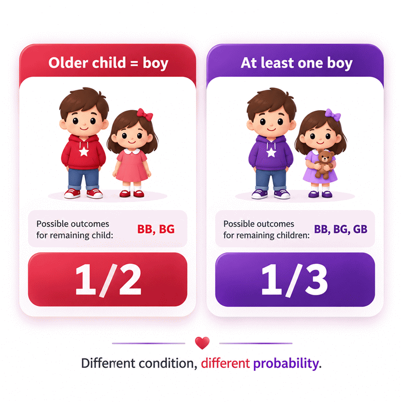
Boy or Girl Paradox Calculator makes the key distinction visible: the answer depends on the information process, not only the family description. When a family is selected because at least one child is a boy, the classic eligible outcomes are BB, BG, and GB. Only BB has two boys, giving the familiar 1/3 result. When the older child is specifically identified as a boy, only BB and BG remain, so the result becomes 1/2.
- The wording defines the conditioning event.
- Family selection and child observation are different experiments.
- BB, BG, GB, and GG form the classic ordered sample space.
- Custom probability mode shows how unequal base probabilities change the model.
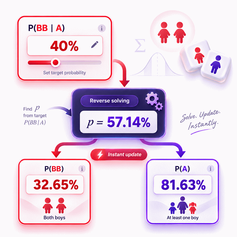
- Editable results allow reverse solving of the underlying probability.
- The sample-space view helps reveal why an intuitive answer can fail.
- AxiCalculator lets users compare scenarios without changing unrelated settings.
The Boy or Girl Paradox Calculator is most useful when you compare scenarios instead of memorizing one percentage. Define how the information was obtained, inspect the surviving outcomes, and then interpret the result.
Assumptions used in this calculator
- The model considers exactly two children in each family.
- Classic mode assigns equal boy and girl probabilities.
- Custom mode applies one boy probability to both births.
- The two children’s outcomes are treated as statistically independent.
- Birth order matters only when the older child is identified.
- At-least-one-boy conditioning excludes the girl-girl family outcome.
- Family-selection conditioning uses probabilities of eligible family types.
- Random-child observation conditions on the child actually observed.
- Sampling method can change the conditional probability result.
- Intermediate probability values are never rounded during calculation.
- Percent and decimal units represent the same probability.
- Reverse solving assumes the edited result matches the selected scenario.
- Real-world birth ratios may differ from model assumptions.
Results are rounded for display.
Internal calculations use full precision.
Formulas Used in Boy or Girl Paradox Variables :
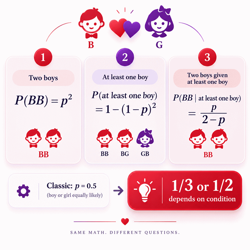
Prior Probability of Two Boys
p is the probability that one child is a boy, and BB is the event that both children are boys.
Probability of At Least One Boy
A is the event that at least one of the two children is a boy.
Identified or Randomly Observed Boy Conditional Probability
O means the older child is identified as a boy, while R means a randomly observed child is a boy.
Family-Selection Conditional Probability
This condition applies when a family is selected after establishing that at least one child is a boy.
Reverse Solve from Two Boys Probability
This reverse equation recovers the underlying boy probability from an edited P(BB) result.
Reverse Solve from At Least One Boy Probability
This reverse equation recovers p from an edited probability of at least one boy.
Reverse Solve from Family-Selection Conditional Probability
This equation recovers p when the family-selection conditional result is edited directly.
Variables & Definitions
View a complete list of all variables used in this calculator, including definitions and units
Boy or Girl Paradox Variables and Probability Definitions
| Symbol | Variable or Event | Meaning | Valid Range |
|---|---|---|---|
| p | Boy probability | Probability that one child is a boy. | 0 < p ≤ 1 |
| BB | Both boys event | Both children in the two-child family are boys. | Event |
| A | At least one boy event | One or both children are boys. | Event |
| O | Older child boy event | The identified older child is known to be a boy. | Event |
| R | Random observed boy event | A randomly observed child is known to be a boy. | Event |
| P(BB) | Prior two-boys probability | Probability that both children are boys before conditioning. | 0 < P(BB) ≤ 1 |
| P(A) | At-least-one-boy probability | Probability that the family contains at least one boy. | 0 < P(A) ≤ 1 |
| P(BB | O) | Older-child conditional probability | Probability of two boys when the older child is identified as a boy. | 0 < P(BB | O) ≤ 1 |
| P(BB | A) | Family-selection conditional probability | Probability of two boys after conditioning on at least one boy. | 0 < P(BB | A) ≤ 1 |
| P(BB | R) | Observed-child conditional probability | Probability of two boys after randomly observing a boy. | 0 < P(BB | R) ≤ 1 |
Unit Conversion Table
Probability Percentage Unit Conversion
| Unit Group | Unit Name | Symbol | Equivalent in Decimal | Used For |
|---|---|---|---|---|
| Popular Units | Percent | % | 1% = 0.01 | User-friendly probability inputs and displayed results |
Decimal Probability Unit Conversion
| Unit Group | Unit Name | Symbol | Equivalent in Percent | Used For |
|---|---|---|---|---|
| Scientific Units | Decimal Probability | 1 | 1.0 = 100% | Probability formulas, scientific notation, and internal calculations |
Example Calculation
The custom boy probability is applied independently to both children.
The girl-girl outcome is excluded by the at-least-one-boy condition.
The remaining probability mass is used to calculate the conditional result.
A denotes the event that the family contains at least one boy.
The conditional output is treated as the known value instead of p.
The reverse equation reconstructs the underlying boy probability first.
Every dependent probability is then recalculated from the recovered p value.
Substitution confirms that P(BB | A) returns exactly 40% before display rounding.
Results are rounded for display.
Internal calculations use full precision.
Calculations Disclaimer
Why 1/3 and 1/2 Can Both Be Correct
A student sees two answers and assumes one must be wrong. That reaction is understandable. The Boy or Girl Paradox looks like one simple question. Yet the wording can describe two different experiments. That difference changes the evidence before any arithmetic begins.
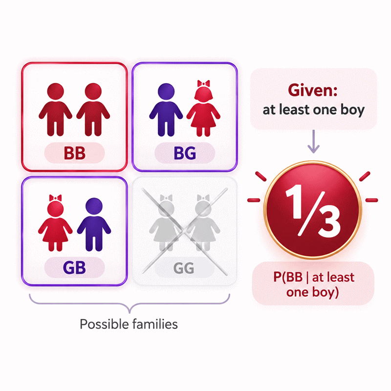
Consider a family with two children. You learn that at least one is a boy. This statement describes the family as a whole. It does not identify either child. Under the classic model, three ordered family types remain possible. They are BB, BG, and GB. Only one contains two boys. That produces the familiar one-third result.
Now change one sentence. You learn that the older child is a boy. The information is now attached to one identified child. Two family types remain. They are BB and BG. One contains two boys. The result is therefore one-half.
The arithmetic did not suddenly become inconsistent. The evidence changed. That is the central lesson. Conditional probability responds to the exact event you know.
This distinction matters because natural language often hides the experiment. People hear “one child is a boy.” They imagine a particular child. The formal condition may instead mean “at least one boy exists.” Those statements sound close. Their mathematical meaning is not identical.
The safest approach is simple. Define how the information was obtained first. Then identify which outcomes remain possible. Only then should you calculate.
AxiCalculator makes this difference visible instead of hiding it. You can switch between scenarios directly. The result changes with the information model. That makes the paradox easier to inspect and harder to memorize incorrectly.
This is also why the problem remains useful. It is not merely a recreational puzzle. It teaches a basic statistical habit. Evidence needs a defined collection process. Without that process, a conditional question may remain ambiguous.
The useful question is therefore not only, “What do we know?” Ask another question first. “How did we learn it?” That second question often controls the answer.
The Condition Changes the Sample Space Before Any Calculation
A learner often starts calculating too early. That creates the first major error. The condition should reshape the possible outcomes before numbers are combined.
Start with four ordered family types. They are BB, BG, GB, and GG. The first position can represent the older child. The second position can represent the younger child. This order matters because BG and GB describe different ordered families.
Suppose the condition says at least one child is a boy. GG cannot satisfy that statement. The other three families can. The conditioned sample space therefore contains three family types.
Now suppose the older child is known to be a boy. Any family beginning with G is impossible. GB and GG disappear. Only BB and BG remain.
This change happens before the final probability is evaluated. That point is easy to miss. Many incorrect solutions keep the wrong sample space and then apply correct arithmetic.
The paradox becomes much less mysterious when outcomes stay visible. A table works well. A probability tree works too. The important step is filtering outcomes with the exact condition.
There is another useful detail. Equal-looking outcomes should only be counted equally when the model supports that treatment. In the classic setup, the standard four outcomes have matching prior weights. That makes direct counting possible after the condition is applied.
Different observation procedures can change those weights. A randomly observed child creates a different evidence process. A family selected because it contains a boy creates another process. The final statement can sound similar while the likelihood of producing that statement differs.
This is why sample-space thinking is more powerful than memorizing one-third. Memorization fails as soon as the question changes. A visible sample space adapts.
Use AxiCalculator as a checking tool rather than an answer box. Select a scenario. Watch which interpretation applies. Then compare the result with your own reasoning. That workflow builds transferable probability skill.
Family Selection and Child Observation Are Different Experiments
A real difficulty appears when someone says, “I saw a boy.” That statement sounds equivalent to “the family has a boy.” It is not always equivalent.
Imagine selecting families because they satisfy a family-wide condition. Every eligible family enters through the same rule. A mixed family qualifies because one child is a boy. A two-boy family also qualifies. The condition filters family types.
Now consider observing one child at random. The evidence comes from a child-level observation. A two-boy family always produces a boy observation. A mixed family produces one only when the observed child is the boy.
The information mechanism has changed. That affects how strongly different family types contribute to the observation.
This idea is central to conditional probability. Evidence is not always a passive sentence. The process producing the evidence can carry information.
Analysts meet the same issue elsewhere. A survey response depends on who was sampled. A defect report depends on how products were inspected. A medical test result depends on the testing process. The details differ, but the reasoning habit is similar.
The Boy or Girl Paradox compresses this lesson into four simple family outcomes. That makes it useful for students and professionals.
The safest workflow is to separate three layers. First, define the underlying possibilities. Second, define how information is generated. Third, evaluate the target event after receiving that information.
Confusion usually comes from skipping the second layer. People jump from a sentence to an answer. They never ask how that sentence became available.
AxiCalculator separates the family-selection interpretation from the observed-child interpretation. This prevents the interface from pretending the wording has one universal meaning.
That separation is more valuable than another decimal place. Precision cannot rescue a poorly defined event. A clear information model can.
When two people disagree about this paradox, check their experiments first. They may be solving different problems. Once their information processes match, the apparent contradiction often disappears.
What the Boy or Girl Paradox Calculator Is Really Testing
A user may expect a calculator to return one fixed percentage. That would hide the most important part of this problem. The calculator should test the relationship between evidence and probability.
Classic mode starts with the familiar balanced setup. This is useful for learning. It keeps attention on the conditioning rule rather than changing base rates.
One scenario identifies the older child. Another describes at least one boy. A separate information model can represent a randomly observed child. These choices are not cosmetic. Each one defines a different experiment.
The result cards should therefore be read together. The prior chance of two boys provides context. The chance of at least one boy provides another layer. The conditional result answers the selected question.
This arrangement helps users see that probability is a connected model. A changed input should affect every dependent result consistently.
The visual sample space supports the same goal. It shows which states survive the selected condition. A user can compare the picture with the numeric result. That creates a fast verification loop.
There is also educational value in editable results. Traditional calculators move only from inputs to outputs. That can encourage passive use. An editable result lets the user ask the opposite question.
Suppose you require a particular conditional probability. What underlying base probability would create it? Reverse solving answers that kind of question. The calculator becomes exploratory rather than one-directional.
This design also catches misunderstandings. An entered result may imply a different base probability than expected. The user can inspect the scenario again. That creates productive friction instead of silently accepting a mistaken assumption.
AxiCalculator should therefore be viewed as a model-testing interface. It computes quickly, but speed is not the main value. The stronger value is transparency.
Use the controls deliberately. Change one condition at a time. Keep the base probability fixed while comparing information models. Then change the base probability. Watch how the whole model responds.
This method turns a famous puzzle into a small probability laboratory. The user does not need advanced software. The logic remains visible on the page.
What Changes When the Base Probability Is Not 50/50
A student often assumes the paradox only works with a balanced 50/50 setup. The underlying structure is more general. A custom base probability changes the weights of the family types.
This matters because BB, BG, GB, and GG no longer share identical probabilities. Directly counting surviving labels is no longer sufficient. Their weights must also be respected.
The conceptual workflow remains unchanged. Define the base probability. Build the family distribution. Apply the condition. Then evaluate the target event inside the conditioned model.
The identified-child scenario remains easy to interpret. Once one child is fixed, uncertainty remains about the other child. Its probability follows the selected base model.
The family-wide condition behaves differently. It filters all families with no boys. The relative weight of BB compared with mixed families changes as the base probability moves.
This makes custom mode useful for learning. It shows which parts of the paradox depend on symmetry. It also shows which parts come from conditioning itself.
Try moving the base probability gradually. Watch the prior values first. Then watch the family-selection result. The relationship becomes easier to understand when it changes continuously.
Do not treat custom mode as a statement about actual demographics. It is a mathematical control. Its purpose is to reveal the structure of the model.
This feature also prevents a common educational mistake. Students sometimes learn the value one-third without learning why it appears. A changing base probability breaks that memorization pattern.
The more useful lesson is procedural. Define probabilities first. Keep the model consistent. Condition only after the underlying distribution is clear.
AxiCalculator makes that procedure visible in real time. That creates a better bridge toward Bayesian reasoning. Users can see that posterior results depend on both prior structure and evidence.
Why Reverse Solving Is More Than a Convenience
A user sometimes knows the desired result but not the underlying probability. A one-way calculator cannot answer that question directly. Reverse solving can.
Reverse solving changes the role of a displayed result. It is no longer a passive label. It can become a known value used to recover the missing model input.
This is particularly useful for validation. Enter a result you believe is correct. The calculator recovers the implied base probability. Compare that value with your original assumption.
If the recovered value differs, something deserves review. The issue may be the scenario. It may be the observation model. It may be an intuitive answer that belongs to another experiment.
This approach is valuable because conditional-probability errors are often structural. They do not come from difficult arithmetic. They come from using the wrong conditioning event.
A reverse-enabled calculator exposes that structure. All displayed values must agree with one underlying model. Changing one value forces the others to update.
That makes reverse solving a consistency check. It can reveal whether a proposed answer belongs to the selected interpretation.
Students can use this as a challenge. Predict the implied base probability before editing a result. Then compare the prediction with the calculator.
Teachers can use the same feature during demonstrations. Analysts can use it to inspect how sensitive a conditional result is to its underlying probability.
The key benefit is not convenience alone. It is model visibility. A one-way answer can hide relationships. Reverse solving brings them to the surface.
AxiCalculator should preserve this behavior across related statistics tools. Consistent reverse interaction can become a recognizable platform feature.
Common Reasoning Traps That Change the Answer
A learner often says, “One child is a boy, so only the other matters.” That statement hides a crucial assumption. It treats the boy as already identified.
If the condition merely says at least one child is a boy, no position was fixed. A mixed family can place the boy first or second. Both ordered outcomes matter.
Another trap is ignoring the information process. Users may compare a family-level statement with a child-level observation. The words sound related. The evidence is generated differently.
A third mistake is counting outcomes without checking their weights. Simple counting is safe only when the relevant outcomes carry the correct equal weight. Custom base probabilities can break that symmetry.
A fourth error is confusing independence with unchanged conditional probability. The two child outcomes can be independent. Yet learning a condition about the pair still changes which families remain possible.
A fifth trap is treating the paradox as a fact about real families. It is primarily a probability model. The classic setup simplifies reality to teach conditional reasoning.
A sixth error is trusting an isolated answer. A percentage without a scenario is incomplete here. The user needs to know which information rule produced it.
A seventh mistake is arguing about one-third and one-half without defining the experiment. Both parties may have correct mathematics for different scenarios.
The solution is procedural. State the experiment. Name the condition. List or weight the remaining outcomes. Then calculate.
This method works beyond the Boy or Girl Paradox. It also helps with medical tests, survey sampling, quality inspection, and screening problems.
The shared principle is selection. Evidence changes what remains plausible. The way evidence appears can also influence that change.
AxiCalculator reduces these mistakes by keeping the scenario visible beside the result. That design choice matters. It prevents a number from becoming detached from its meaning.
How to Use AxiCalculator to Test the Paradox Yourself
A user may understand the explanation but still distrust the surprising result. The best response is to test the model directly.
Start with the classic probability setting. Choose the older-child scenario first. Observe the conditional result. Then switch to the at-least-one-boy scenario.
Keep every other setting unchanged. Only the information condition should move. This isolates the effect of the wording.
Next, inspect the sample space. Notice which family types disappear in each scenario. The numeric change should now match a visible structural change.
Then switch the information model. Compare family selection with random child observation. Focus on how the evidence was generated.
After that, enter a custom base probability. Do not try to predict everything at once. Watch the prior family values first. Then inspect the conditional result.
Finally, edit one calculated result. Let the reverse solver recover the base probability. Compare the recovered model with your expectation.
This sequence is more useful than memorizing a single answer. It creates a repeatable reasoning process.
The same approach can help with other probability tools. Change one condition at a time. Watch the sample space. Check whether evidence is family-level or observation-level.
AxiCalculator also lets you share the configured result. That helps when discussing the paradox with classmates or colleagues. Both people can inspect the same scenario instead of arguing from different hidden assumptions.
Export features are useful when results need to accompany coursework or internal notes. The calculation remains easier to audit when the selected scenario is preserved.
The final goal is simple. Do not ask the calculator to replace reasoning. Use it to test reasoning.
When the result looks surprising, inspect the information process first. When two answers disagree, compare their conditioned events. When a wording change changes the result, treat that as information rather than a contradiction.
The Boy or Girl Paradox becomes much easier once those habits are automatic. What first looks like a trick becomes a clear lesson in conditional probability. AxiCalculator turns that lesson into something users can manipulate, verify, and understand.
Frequently Asked Questions
Why can 1/3 and 1/2 both be correct?
Does birth order always matter in the Boy or Girl Paradox?
Does this calculator predict the composition of a real family?
What happens when the base probability is not 50%?
How should an analyst define the sampling mechanism before calculating?
When is counting surviving outcomes mathematically unsafe?
How can reverse solving help validate a conditional probability model?
Engineering Resources
Our engineers are here to help you get it right.