Coin Flip Probability Calculator
- Last formula update:
Decimal & Rounding Policy
- Input values are normalized before calculation without intermediate rounding.
- Binomial terms and cumulative probabilities retain full calculation precision.
- Displayed results use up to 12 significant digits where practical.
- Percentage results are converted from the unrounded decimal probability.
- Reciprocal probability is calculated as 1 divided by the unrounded probability.
- Rounding affects display only and never changes the underlying result.
Valid range
- Number of flips: whole numbers from 1 to 10000.
- Number of heads: whole numbers from 0 through the number of flips.
- Probability of heads: 0 to 1 in decimal form.
- Probability of heads: 0% to 100% when percentage units are selected.
- Probability of heads: 0 to 1000000 ppm when ppm units are selected.
- An empty heads probability uses 0.5 for forward calculation.
- Calculated probability: 0 to 1 inclusive.
- Chance of success: 0% to 100% inclusive.
- Probability of 1 in N: N is at least 1, or Infinity when probability is zero.
- Reverse solving requires exactly one of n, k, or p to be unknown.
- Reverse number-of-flips search supports unique integer solutions through 2000 flips.

Wylena Brantford
Reviewers:
Valdren Clyforde
Zenara Dentwick
Check our editorial policy
September 22, 2026
1.0.0
Initial calculator and formula release.
Our engineers are here to help you get it right.
How Does a Coin Flip Probability Calculator Turn Repeated Tosses Into Reliable Odds?
Coin Flip Probability Calculator results show how likely a selected head-count event is across repeated independent flips. The tool can evaluate exactly, at least, or at most a chosen number of heads while supporting both fair and biased coins. A Coin Flip Probability Calculator is most useful when the event wording, number of flips, target heads, and heads probability are defined correctly.
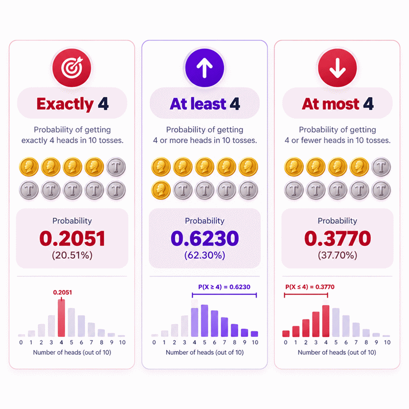
- Exactly counts only the selected number of heads.
- At least includes the selected count and every larger valid count.
- At most includes the selected count and every smaller valid count.
- A fair coin uses an equal heads and tails chance.
- A biased coin shifts probability toward its favored outcome.
- Independent flips do not remember previous results.
- A head count differs from one exact ordered sequence.
- Expected heads describe a long-run average, not a guaranteed count.
- Reverse solving can find one missing input when a unique solution exists.
- Some reverse problems have no solution or multiple valid solutions.
- Percentage and 1-in-N views express the same underlying probability differently.
- Always interpret the output together with the selected event type.
Assumptions used in this calculator
- Each flip has exactly two mutually exclusive outcomes.
- Coin flips are treated as statistically independent trials.
- Probability of heads remains constant across all flips.
- A fair coin uses a heads probability of 0.5.
- Biased coins use the user-entered heads probability.
- Number of flips is a positive whole number.
- Number of heads ranges from zero through total flips.
- Probabilities are normalized to decimal form before calculation.
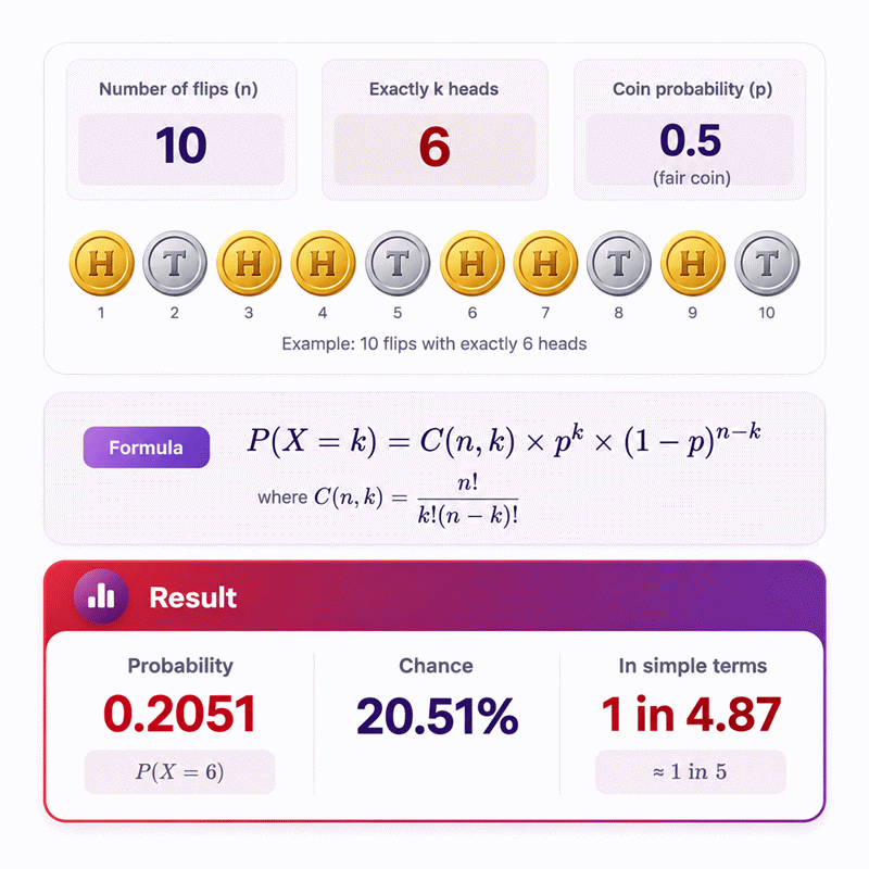
- Exact results follow the binomial probability mass function.
- At-most results sum probabilities through the selected head count.
- At-least results sum probabilities from the selected head count.
- Reverse solving assumes exactly one calculator variable is unknown.
- Display rounding never changes internal calculation precision.
Results are rounded for display.
Internal calculations use full precision.
Formulas Used in Coin Flip Probability Calculator :
Binomial Coefficient
Probability of Exactly i Heads
Probability by Selected Mode
Probability Unit Normalization
Result Display Conversions
When R = 0, the reciprocal 1-in result is Infinity.
Reverse Solving Equation
Exactly one of n, k, or p is treated as unknown.
The probability p is solved on 0 ≤ p ≤ 1 when a unique solution exists.
The values n and k are solved only as valid whole-number solutions.
n = total number of flips.
k = requested number of heads.
i = summation index for possible head counts.
p = probability of heads on each independent flip.
C(n, i) = number of combinations containing i heads among n flips.
qi = probability of obtaining exactly i heads.
m = selected calculation mode: exactly, at most, or at least.
R = final decimal probability of the selected event.
Rtarget = user-entered probability used for reverse solving.
N1-in = reciprocal representation of the final probability.
All intermediate calculations retain full available precision; rounding is display-only.
Variables & Definitions
View a complete list of all variables used in this calculator, including definitions and units
Coin Flip Probability Calculator Variables and Symbols
| Symbol | Meaning | Valid Range or Type | Unit or Representation |
|---|---|---|---|
| n | Total number of coin flips | Whole number, 1 to 10000 | Flips or trials |
| k | Requested number of heads | Whole number, 0 to n | Heads or successes |
| i | Summation index for possible head counts | Whole number within the active summation | Count |
| p | Probability of heads on one flip | 0 to 1 inclusive | Decimal probability |
| C(n, i) | Number of combinations with i heads among n flips | Positive combinatorial value | Dimensionless |
| qi | Probability of exactly i heads | 0 to 1 inclusive | Decimal probability |
| m | Selected probability mode | Exactly, at most, or at least | Mode |
| R | Final probability of the selected event | 0 to 1 inclusive | Decimal probability |
| Rtarget | Target result entered during reverse solving | 0 to 1 inclusive | Decimal probability |
| N1-in | Reciprocal representation of the event probability | 1 or greater, or Infinity when R equals 0 | 1 in N |
Unit Conversion Table
Coin Flip Probability Calculator Unit Conversion Table
| Unit Group | Unit Name | Symbol | Equivalent in Base Unit | Used For |
|---|---|---|---|---|
| Popular Units | Flip | flips | 1 flip = 1 trial | Total number of coin tosses |
| Scientific Units | Trial | trials | 1 trial = 1 flip | Total number of Bernoulli trials |
| Popular Units | Head | heads | 1 head = 1 success | Number of heads obtained or required |
| Scientific Units | Success | successes | 1 success = 1 head | Binomial success count |
| Popular Units | Decimal Probability | decimal | 1 decimal = 100% | Probability input and internal calculations |
| Popular Units | Percent | % | 1% = 0.01 decimal | User-friendly probability and chance display |
| Scientific Units | Parts Per Million | ppm | 1 ppm = 0.000001 decimal | Very small probability values |
| Popular Units | One in N | 1 in N | Decimal probability = 1 / N | Reciprocal probability representation |
Example Calculation
The calculation asks for exactly seven heads in twelve independent flips.
Each head has probability 0.60, while each tail has probability 0.40.
The combination factor counts every arrangement containing seven heads.
The final event probability is approximately 22.703%.
The target result represents getting at least one head.
The complement event is obtaining tails on every flip.
Reverse solving isolates the unknown number of independent flips.
The unique whole-number solution is five flips.
Results are rounded for display.
Internal calculations use full precision.
Calculations Disclaimer
How Should You Read a Coin Flip Probability Result?
A probability result can look precise while still being misunderstood. The Coin Flip Probability Calculator solves that problem by separating event types clearly. The Coin Flip Probability Calculator also lets you compare results without manual combinatorial work. A decimal such as 0.25 means the same thing as 25 percent. Yet the event behind that number matters just as much.
First identify what the result describes. An exact result covers one head count. An at-least result covers that count and every larger count. An at-most result covers that count and every smaller count. These events can produce very different answers from identical inputs.
The number of flips controls how many trials occur. The head count defines the event boundary. The probability of heads controls how likely each head is. A fair coin uses equal head and tail chances. A biased coin shifts the distribution toward one side.
Do not read a probability as a prediction of what must happen. It measures uncertainty before the experiment. A 70 percent event can fail. A 2 percent event can occur. Probability describes likelihood, not destiny.
READ THE RESULT IN THIS ORDER:
EVENT TYPE → INPUTS → PROBABILITY → PRACTICAL INTERPRETATION
This reading order prevents the most common interpretation error. Users often focus on the percentage first. They then forget whether the calculator answered “exactly,” “at least,” or “at most.” The percentage is only meaningful when attached to the correct event.
A useful result should therefore answer two questions. What event did you ask about? How likely is that event under your selected coin model? Once both answers are clear, the number becomes useful rather than merely impressive.
Why Is Exactly k Heads Different From a 50% Chance?
A common problem appears when users expect balanced coins to produce balanced counts every time. A fair coin gives each individual flip equal chances. It does not make every possible head count equally likely. Those are different ideas.
Suppose many flips occur. Several different sequences can contain the same number of heads. Near the middle, many sequences share similar head counts. At the extremes, far fewer sequences exist. That makes middle counts more likely than all-heads or all-tails outcomes.
A fair coin therefore creates a symmetric distribution. Symmetry does not mean every count has equal probability. It means corresponding counts on opposite sides behave symmetrically. The middle receives more combined sequence weight.
This distinction explains a surprising result. Exactly half heads may be the most likely individual count. It still may represent only a modest share of all possible outcomes. Other nearby counts collectively hold substantial probability.
That is why “the coin is 50/50” cannot answer a multi-flip question alone. The 50 percent value describes one trial. A multi-flip event combines repeated trials and possible arrangements. The event definition determines which arrangements belong in the answer.
Users often make a second mistake here. They confuse the expected proportion with a guaranteed count. As the experiment grows, the proportion tends to concentrate near its expected level. However, one precise count remains only one point inside a wider distribution.
The practical lesson is simple. Use the single-flip probability to model each trial. Use the selected event to interpret the complete experiment. Never replace the second idea with the first.
Why Multiple Sequences Can Produce the Same Head Count
A real counting problem begins when order creates several ways to reach one total. Three heads can appear early, late, or between tails. Every arrangement contributes to the event “exactly three heads.” Ignoring those arrangements creates a large error.
The calculator handles the arrangements automatically. That matters because manual enumeration becomes difficult quickly. Ten flips already create many possible sequences. Twenty flips create far more. Yet many of those sequences collapse into the same head count.
This is the key difference between sequence probability and count probability. A sequence identifies every position. A count ignores position and groups sequences together. Those are distinct questions.
Consider the phrase “four heads in eight flips.” It usually means any arrangement containing four heads. It does not normally mean one fixed pattern. A fixed pattern might be HHTHTHTT. The count event contains that pattern and many others.
Language therefore matters before calculation starts. “Exactly four heads” is a count event. “Heads, heads, tails, heads…” is a sequence event. “At least four heads” is a cumulative count event. Each deserves a different interpretation.
QUESTION TYPE
Exact count → combines every sequence with that count
Exact sequence → uses one specified order
At least → combines the target and all larger counts
At most → combines the target and all smaller counts
This mental map prevents an important error. Do not multiply the same single-flip probability repeatedly when the event allows several arrangements. That approach usually calculates one sequence, not the complete count event.
What Does At Least k Heads Really Include?
A user may ask for “at least six heads” and accidentally calculate only six. That misses every outcome with seven, eight, nine, or more heads. The phrase “at least” sets a lower boundary, not one exact target.
The calculator treats the selected count as included. If the target is six, then six qualifies. Every larger valid head count also qualifies. The event continues through the total number of flips.
This becomes especially useful for threshold questions. A student may need the chance of meeting a minimum target. A quality analyst may treat “success” as reaching a minimum count. A simulation designer may care about crossing a threshold. The mathematics follows the same event structure.
At-least probability usually falls as the threshold rises. Requiring one or more heads includes many outcomes. Requiring nearly all heads includes far fewer outcomes. The event becomes stricter.
This behavior gives you a valuable reasonableness check. If you increase the minimum required heads while keeping everything else fixed, the probability should not increase. If it does, recheck the event definition or input values.
A biased coin changes the curve but not the meaning. A coin favoring heads makes high thresholds easier to reach. A coin favoring tails makes them harder. The event still includes the target and every larger head count.
At-least calculations are also where intuitive shortcuts can be useful. Some events have a simple opposite. The probability of one or more heads can be understood by considering the only excluded case: zero heads. This conceptual shortcut often makes the result easier to explain.
When the Complement Method Makes the Answer Easier
A complicated event can become simple when its opposite has fewer possibilities. This is the main reason complement reasoning matters. It reduces counting without changing the underlying event.
“At least one head” is the classic case. Direct counting includes every outcome except all tails. The opposite event is therefore much simpler to describe. Similar logic works for other threshold problems when one tail is shorter than the other.
The complement is not a different probability model. It is another route to the same event. Used correctly, it improves speed and reduces manual mistakes.
However, complements require careful boundary handling. The opposite of “at least k” is “fewer than k.” That means counts below k. The opposite is not “at most k” because that would include k itself.
This single boundary difference causes many student errors. Words such as at least, more than, at most, and fewer than sound similar. They are not interchangeable.
BOUNDARY CHECK
At least k includes k.
More than k excludes k.
At most k includes k.
Less than k excludes k.
When using AxiCalculator, choose the mode that matches the exact wording. Do not choose based on which result “looks right.” Probability problems reward precise event definitions more than intuition.
What Does At Most k Heads Really Include?
A threshold problem can fail because “at most” gets mistaken for “exactly.” At most four heads includes zero, one, two, three, and four heads. It stops at the chosen maximum.
This is a lower-tail event. It answers questions about staying below a ceiling. If the allowed maximum increases, more possible outcomes qualify. The probability therefore cannot decrease while other inputs remain fixed.
That monotonic behavior is useful for checking results. If the at-most probability becomes smaller after raising k, something is inconsistent. Either the inputs changed or the event was misread.
The fair-coin case has another useful pattern. Lower and upper tails mirror each other around the center. Bias breaks that visual symmetry. A head-favoring coin pushes more mass toward larger head counts. A tail-favoring coin pushes it downward.
At-most events appear in more places than classroom coin exercises. They model limits and failure thresholds in repeated yes/no systems. The coin is simply an intuitive representation of a broader discrete-probability structure.
The key is still the same. Trials need a stable success chance. They also need the required independence. If those conditions fail, the numerical result may no longer describe the real process accurately.
How Lower-Tail Probability Changes as k Moves
A user may wonder why a cumulative result grows quickly near the center. The reason is that central head counts can hold substantial probability. Adding one central count can therefore move the cumulative total noticeably.
Far into an extreme tail, each additional count may contribute much less. The cumulative total can then change more slowly. This behavior depends on the coin’s bias and number of trials.
Thinking in distributions makes these results easier to understand. Do not imagine each possible head count as equally sized. Their probabilities vary. The distribution shows how likelihood is allocated across counts.
A fair coin places its center near half the flips. A biased coin moves that center. The cumulative total simply collects the probability from one side through the selected boundary.
This perspective is more useful than memorizing isolated answers. Once you understand movement across the distribution, many results become predictable in direction. That helps detect data-entry mistakes before relying on an output.
How Does a Biased Coin Change the Distribution?
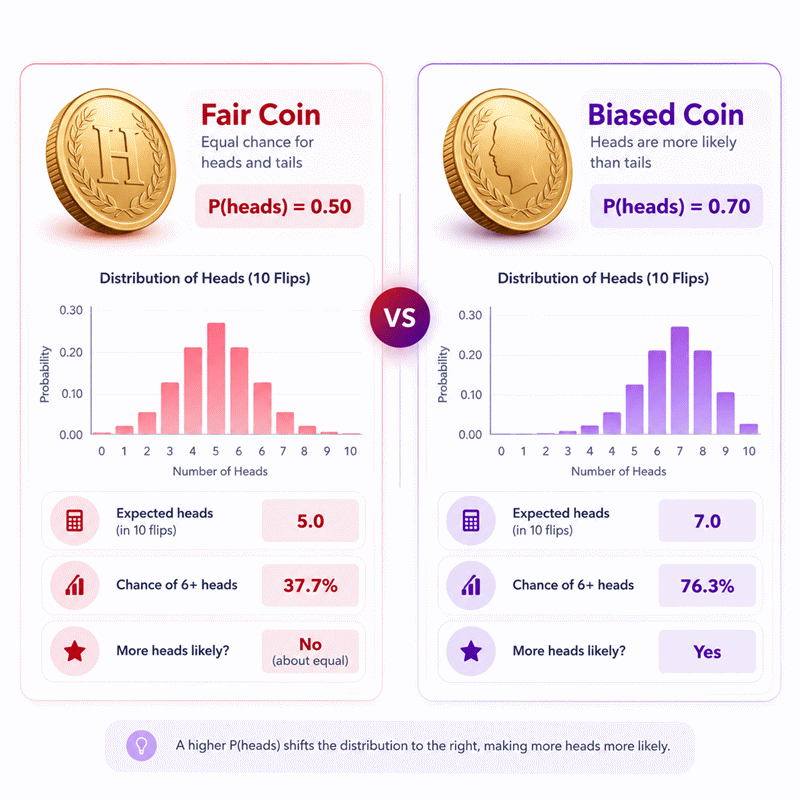
A real experiment may not justify a 50 percent head chance. Using 0.5 anyway creates a model error before calculation even begins. A biased-coin setting solves that problem when the bias is known or intentionally specified.
If heads are more likely, larger head counts become more likely. The distribution shifts upward. If heads are less likely, smaller counts gain probability. The distribution shifts downward.
Bias does not remove randomness. A 70 percent heads coin can still produce tails. It can even produce an unusual run of tails. Bias changes relative likelihood, not possibility.
This is important when interpreting a surprising result. One short sequence cannot reliably reveal the true bias. A calculator answers the probability under a chosen p value. It does not automatically estimate the physical bias from one small observation.
Users should therefore distinguish two tasks. One task predicts outcomes from a known probability. Another task estimates probability from observed data. They are related, but they are not the same question.
The Coin Flip Probability Calculator focuses on the first task. It evaluates events under the probability you provide. Its reverse-solving capability can solve certain mathematical target equations. That still should not be confused with formal statistical estimation.
What Changes When the Probability of Heads Is Not 0.5?
A common misconception says only the center changes. More than the center changes. Every head-count probability responds to the new single-trial chance.
High-head outcomes receive more weight when p rises. Low-head outcomes lose weight. The reverse happens when p falls. The distribution can also become visibly asymmetric.
Threshold probabilities respond strongly. An “at least” event near the upper range can become much more plausible. An “at most” event near the lower range can become less plausible. The exact impact depends on n and k.
Extreme p values create especially concentrated behavior. A probability near one strongly favors head-heavy outcomes. A probability near zero strongly favors tail-heavy outcomes. Boundary values create deterministic cases.
This is why the p field deserves careful attention. Changing it is not a cosmetic setting. It changes the underlying probability model for every flip.
Why Independence Matters More Than the Coin Itself
A calculation can look perfect while modeling the wrong process. Independence is one of the most important hidden requirements. One trial must not change the probability of another.
For an idealized coin model, each toss starts fresh. Previous heads do not consume future heads. Previous tails do not make a head “due.” The next trial keeps the same defined p value.
Real systems can violate this condition. Mechanical processes can drift. Human behavior can adapt. Sampling without replacement can change later probabilities. These situations need different models.
The coin language can therefore be misleading if copied blindly into other fields. The mathematics applies to repeated binary trials only when its structure fits. Two outcomes alone are not enough.
You also need a fixed number of trials for the standard count model. You need a constant success probability. You need independent trials. Once these conditions hold, the binomial framework becomes appropriate.
This matters for professional use. A clean calculator result does not rescue poor assumptions. Good statistical practice begins with model selection, not button pressing.
Why the Gambler’s Fallacy Produces Wrong Predictions
Five tails in a row can create a strong feeling that heads must come next. That feeling is psychologically powerful. It is also wrong under independent fair flips.
The next flip does not compensate for earlier results. Independence means the new trial does not inherit a debt from the sequence. A fair coin remains fair on the next toss.
This does not mean long-term proportions cannot stabilize. They often become less volatile as more trials accumulate. That statistical pattern does not create short-term correction pressure.
Confusing these ideas produces the gambler’s fallacy. People see a streak, expect immediate balance, and change their prediction. The streak itself does not alter the next independent probability.
A probability calculator can help expose this intuition error. Entering the same single-flip p after any history produces the same next-trial chance. What changes is the probability of complete multi-flip events, not the memory of the coin.
PAST STREAK ≠ FUTURE DEBT
Independent trial → same p
Long sequence → many possible patterns
Rare streak → possible, not impossible
Expected balance → long-run concept, not forced correction
What Is the Difference Between a Head Count and an Exact Sequence?
A user asks for three heads and enters a result for one fixed pattern. The answer becomes too small. A head count and a sequence describe different events.
A count cares only about how many heads appear. It does not care where they appear. A sequence specifies the exact order. That difference changes how many outcomes belong to the event.
For a fair coin, every exact sequence of the same length has equal probability. Yet a count may contain many such sequences. That makes the count event much more likely than one chosen sequence.
For a biased coin, sequence probability still depends on the number of heads and tails. Sequences with the same counts share the same probability when p stays constant. The count event then combines all those arrangements.
Before calculating, rewrite the question in plain language. Does it ask “how many?” or “in what order?” That single check often prevents the entire solution from going off course.
Why Order Changes Sequence Probability Questions
A sequence problem can look easier because no combinations are needed. That simplicity is deceptive. It answers a narrower question.
For example, one chosen pattern fixes each flip. A count event allows every ordering matching its total. Using sequence logic for a count discards valid outcomes.
Order also matters when studying streaks. “Seven heads total” differs from “seven consecutive heads.” The first ignores adjacency. The second requires an uninterrupted run.
Do not use a count calculator to answer a streak question unless the event happens to coincide. They represent different structures. A streak tool needs position-aware logic.
AxiCalculator’s coin probability tool should therefore be read as a head-count calculator. Its exact mode means an exact count, not an exact ordered sequence. This wording should stay clear wherever the result is reused.
What Does the Expected Number of Heads Actually Tell You?
A user may see an expected count of five and assume five must occur. Expected value does not make that promise. It describes an average across repeated versions of the same experiment.
If many identical experiments were repeated, their head counts would average toward the expectation. Individual experiments can fall above or below it. Some may differ substantially.
Expected value is useful because it locates the distribution. It gives a simple center for understanding likely counts. It does not describe the full spread.
Two distributions can share a similar center yet behave differently around it. That is why probability questions still need the complete distribution or event calculation.
For a fair coin, expected heads sit at half the flips. A biased coin moves the expected count toward its favored outcome. The change is intuitive, but again not deterministic.
Why the Expected Count Is Not a Guaranteed Result
A practical problem appears when expected value is treated like a forecast. The user then labels every other outcome abnormal. That conclusion is often unjustified.
Random variation is part of the model. Counts around the expected level can all be common. Even noticeably different counts may remain plausible.
The number of trials affects this interpretation. Small experiments can fluctuate widely. Larger experiments often show more stable proportions. Yet exact equality remains unnecessary.
This difference between count and proportion matters. Deviating by five heads has different meaning in ten flips and ten thousand flips. Context changes the scale.
A good interpretation therefore considers n, p, the selected event, and the resulting probability together. One number alone rarely tells the whole story.
What Happens to Coin Flip Probabilities as the Number of Flips Grows?
More flips can create a surprising effect. The proportion of heads may become more stable, while one exact head count becomes less dominant. Both statements can be true.
The reason is scale. More trials create more possible counts. Probability becomes concentrated around the expected proportion, but it spreads across several neighboring integer counts.
This explains why an exact 50–50 split is not guaranteed in a long fair-coin experiment. The region near half becomes increasingly important. One exact count still represents only one point.
Large n also creates numerical challenges. Direct factorial calculations can overflow. Extremely small probabilities can underflow. Stable calculator implementations therefore avoid careless intermediate arithmetic.
For users, the main lesson is conceptual. Do not interpret long-run stabilization as an exact balancing mechanism. Probability becomes more concentrated in proportional terms, not magically deterministic.
Why the Distribution Tightens Without Guaranteeing an Exact Split
A fair coin may produce 49 percent heads, 50 percent, or 51 percent. With many flips, those proportions can all sit close to the same expected center.
The word “tightens” describes relative spread. It does not mean every experiment lands on one integer. Integer counts remain discrete.
This distinction becomes important in quality thresholds and repeated binary tests. A target region can become highly likely even while one exact target stays modest.
Users should therefore choose event wording based on their real goal. If a range is acceptable, an exact-count question may be unnecessarily restrictive. If one precise count matters, exact mode is appropriate.
Probability becomes more useful when the event matches the decision. The calculator cannot choose that decision for you. It can only answer the event you define.
How Can Reverse Coin Probability Solving Find a Missing Input?
A user sometimes knows the desired result but not the input that creates it. Standard calculators stop there. Reverse solving turns the relationship around.
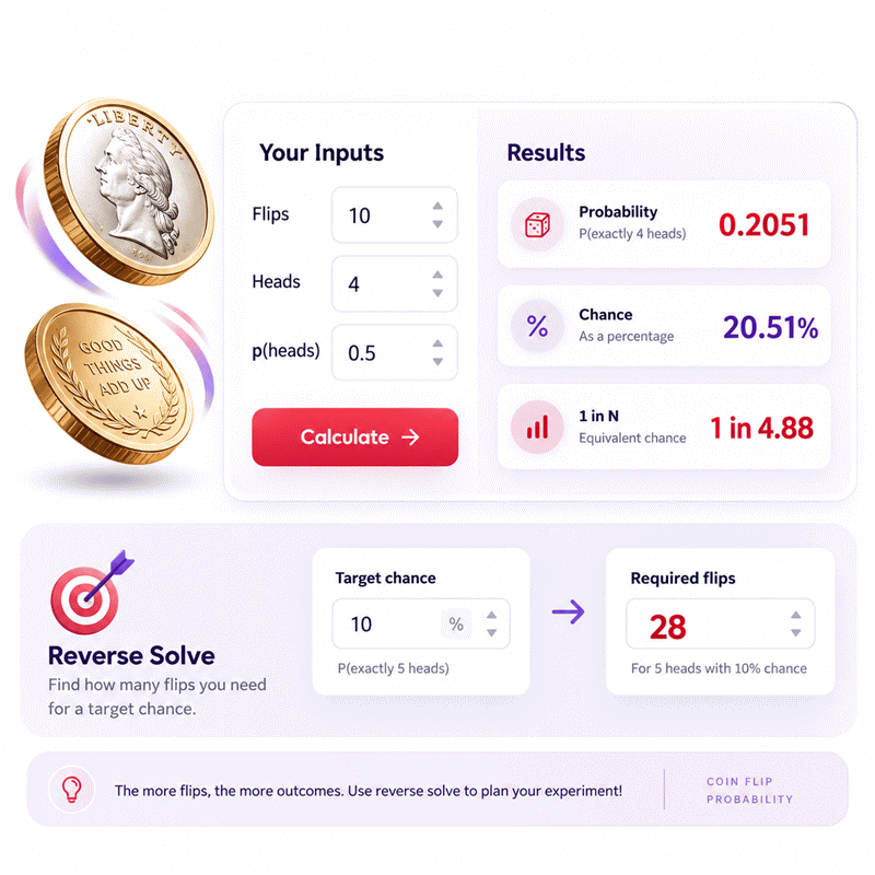
You can leave one compatible variable unknown and enter a target result. The calculator can then search for a missing probability, head count, or flip count when the solution is mathematically identifiable.
This is useful for planning questions. You might know a desired threshold probability. You may want to discover how many trials meet it. You may instead know n and k, then seek the p value that matches a cumulative target.
Reverse solving deserves stricter validation than forward calculation. Counts must remain integers. The head count cannot exceed flips. Probability must remain inside its valid interval.
Not every target produces a valid answer. Some targets fall between values available to a discrete integer variable. Other targets can correspond to several solutions. A trustworthy tool should report that instead of inventing one.
Why Some Reverse Probability Problems Have Multiple Solutions
A reverse problem can look simple and still be ambiguous. Exact-count probability may rise as p approaches a favorable region, then fall afterward. A target value can cross that curve twice.
This means two different coin biases can sometimes produce the same exact-event probability. Selecting one silently would be misleading.
Cumulative events often behave more simply. Their probability may change monotonically with p under ordinary valid boundaries. That can support a unique numerical solution.
Integer reverse problems have another challenge. The desired probability may sit between two possible counts. No exact integer solution then exists.
A robust reverse calculator should distinguish “no solution” from “multiple solutions.” Those are mathematically different outcomes. Both are more useful than a forced answer.
How Should Very Small Coin Flip Probabilities Be Interpreted?
A tiny percentage can trigger an emotional reaction. Users may call the event impossible. That word is usually too strong.
A nonzero probability means the event remains possible under the model. It may be rare, but repetition creates opportunities for rare outcomes to appear.
Scale matters. A one-in-a-million event is unlikely in one attempt. Across millions of opportunities, observing such events becomes far less surprising.
This is why small probabilities should not be interpreted without exposure count. The calculator gives event probability for the defined experiment. It does not automatically tell you how often the experiment occurs in the real world.
Likewise, seeing a rare outcome does not prove the model is wrong. It may justify further investigation. One observation alone usually cannot establish bias or manipulation.
When Percentage and 1-in-N Views Make Results Easier to Understand
A decimal such as 0.0005 can be hard to grasp quickly. Percentage and reciprocal views translate the same probability into familiar formats.
Percentage works well for ordinary probabilities. People generally understand 25 percent faster than 0.25. Very small percentages can still feel abstract.
A 1-in-N view can make rarity more intuitive. It expresses the reciprocal scale of a nonzero event. This does not create a new probability. It simply changes presentation.
Users should avoid interpreting “1 in N” as a schedule. A 1-in-100 event is not guaranteed once every 100 trials. Independent randomness can create clusters and long gaps.
Presentation should improve comprehension without changing meaning. AxiCalculator can show multiple views so users can choose the one that communicates best.
Which Coin Flip Probability Mistakes Cause the Biggest Errors?
The biggest errors usually begin before arithmetic. The event gets defined incorrectly. A flawless calculation then answers the wrong question.
The first mistake is confusing exactly with at least. The second is confusing count probability with sequence probability. The third is assuming past flips change future independent flips.
Another mistake is forcing a fair-coin assumption onto a biased-coin problem. If p differs from 0.5, using 0.5 changes every relevant probability.
Users also confuse theoretical and experimental probability. A short observed run can differ substantially from a theoretical probability. That does not automatically invalidate the model.
Reverse solving adds two more traps. One is assuming every target has an integer solution. The other is assuming every probability target identifies one unique p.
FAST ERROR CHECK
Did I choose the correct event?
Is p correct?
Are the trials independent?
Is k between zero and n?
Am I asking for a count or a sequence?
These checks take seconds. They prevent errors that no extra decimal precision can repair.
How Can You Check a Result Before Trusting It?
A surprising result should trigger verification, not immediate rejection. Start with boundary logic. Every probability must remain between zero and one.
Next test easy cases. Zero required heads, all required heads, or one flip can provide intuitive checks. Symmetry can help when the coin is fair.
Then inspect direction. Raising an at-least threshold should not increase its probability. Raising an at-most threshold should not decrease its probability.
Check the coin bias. A larger head probability should generally shift likelihood toward larger head counts. If the behavior seems reversed, recheck the input.
Finally, confirm the wording. Many “wrong calculator” reports are actually event-definition mismatches. Exactly, at least, at most, and sequence questions can differ dramatically.
AxiCalculator is most valuable when it shortens verification rather than replacing thought. Use the immediate result, then apply these simple sanity checks.
Where Can Coin Flip Probability Reasoning Be Applied Beyond Coins?
A workplace problem may contain no physical coin at all. The same reasoning still applies when repeated trials have two outcomes. That makes this calculator useful as a learning model for broader probability work.
A trial could mean pass or fail. It could mean defect or no defect. It could mean response or no response. The labels do not matter mathematically.
The structure does matter. The number of trials must be fixed for the standard count question. Outcomes must fit two categories. Success probability must stay constant. Trials must remain independent.
When those conditions hold, the head count becomes a general success count. The coin simply makes the model easier to visualize.
When those conditions fail, another distribution may be more appropriate. Sampling without replacement can change probabilities. Time-varying processes can change p. Dependent events require different treatment.
This is the deeper value of the tool. It teaches users to recognize a statistical structure, not merely solve a coin puzzle. A clear model can then support classroom work, experiments, simulations, testing, and other repeated binary processes.
AxiCalculator keeps that workflow practical. Define the event first. Enter the known values. Read the result in context. Reverse-solve only when one missing quantity is identifiable. Then verify whether the real process actually matches the model.
Frequently Asked Questions
Can a fair coin produce a very unbalanced result without being defective?
Why does the same number of heads have different probabilities with different flip counts?
Is getting 50% heads the same as getting exactly half heads?
Can I use this calculator when the probability of heads is unknown?
Why can reverse solving an exact probability produce two valid p values?
When should I stop using a binomial coin model for a real process?
Why can large-n calculations need more careful numerical methods?
Our engineers are here to help you get it right.