Bertrand’s Paradox Variables and Calculation
- Last formula update:

Decimal & Rounding Policy
- All calculations use available JavaScript floating-point precision before display formatting.
- Intermediate radius, threshold, ratio, and probability values are never rounded.
- Length inputs are converted to meters internally before formulas are evaluated.
- Probability calculations use decimal values internally, regardless of the selected display unit.
- Displayed probabilities use up to 10 significant digits and omit unnecessary trailing zeros.
- Reverse calculations always use unrounded source values to minimize cumulative numerical error.
Valid range
- Circle radius R: greater than 0, with a supported base range from 1e-12 m to 1e15 m.
- Chord threshold L: 0 or greater, with a supported base maximum of 2e15 m.
- Custom forward calculation requires the chord threshold to satisfy 0 <= L <= 2R.
- Probability P: 0 to 1 in decimal form, equivalent to 0% through 100%.
- Reverse radius solving requires L > 0 and 0 <= P < 1.
- Reverse threshold solving accepts 0 <= P <= 1 for a positive finite radius.
- Classic mode uses L = sqrt(3)R, which always remains below the circle diameter.

Wylena Brantford
Reviewers:
Valdren Clyforde
Zenara Dentwick
Check our editorial policy
September 20, 2026
1.0.0
Initial calculator and formula release.
Our engineers are here to help you get it right.
Why Does the Bertrand’s Paradox Calculator Give Different Random Chord Probabilities?
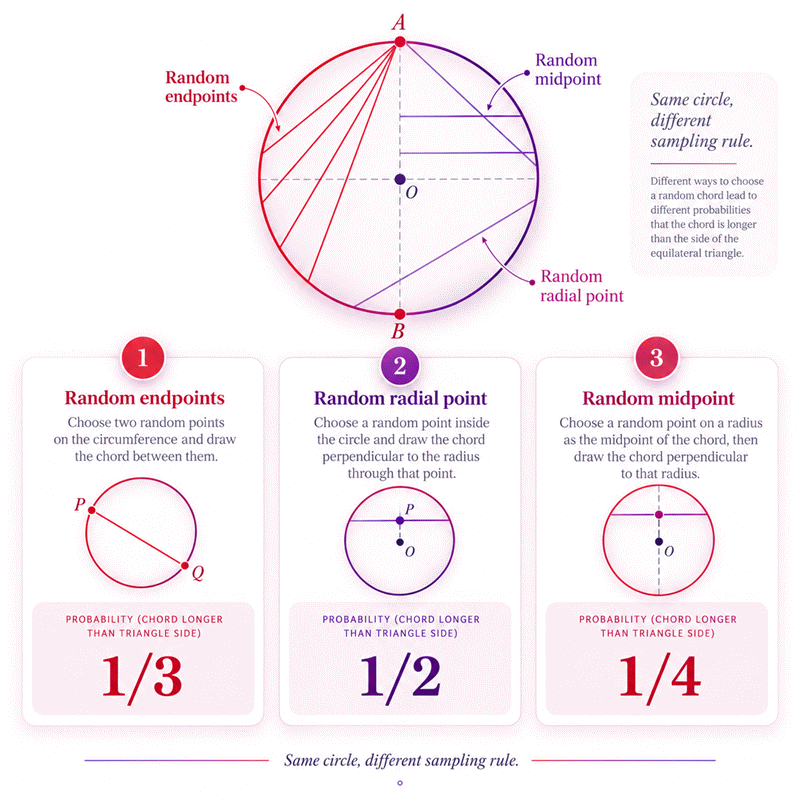
Bertrand’s Paradox Calculator shows that a random chord has no single probability model until the sampling method is defined. The same circle and chord threshold can therefore produce different valid results.
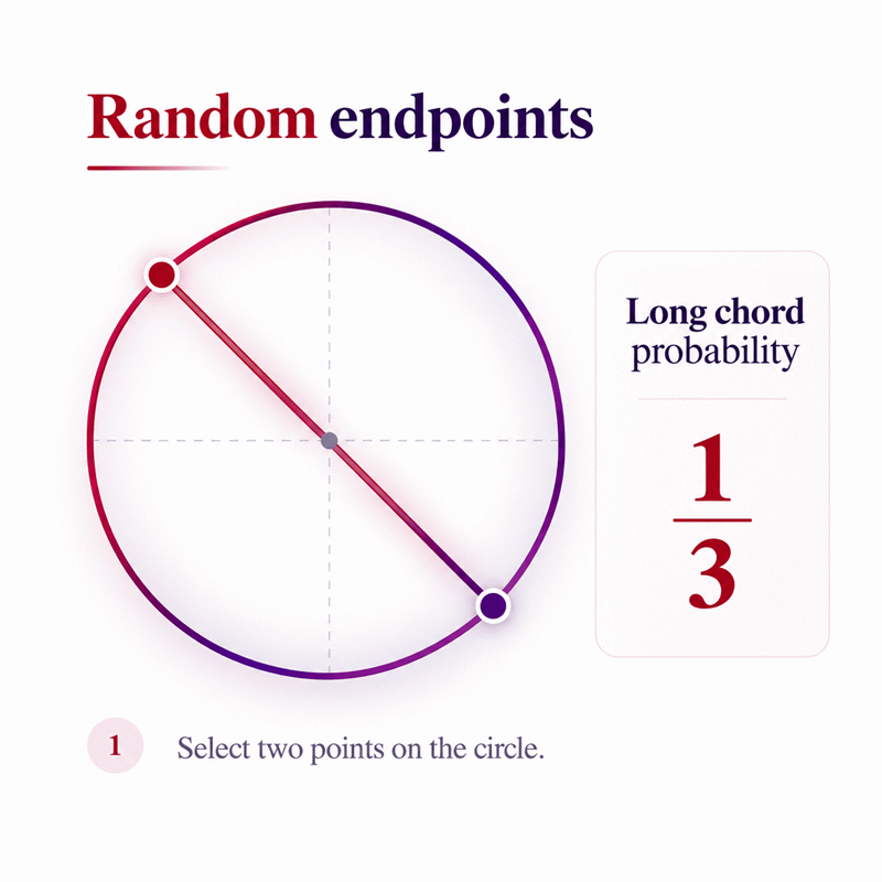
- Random endpoints produce the classic one-third probability.
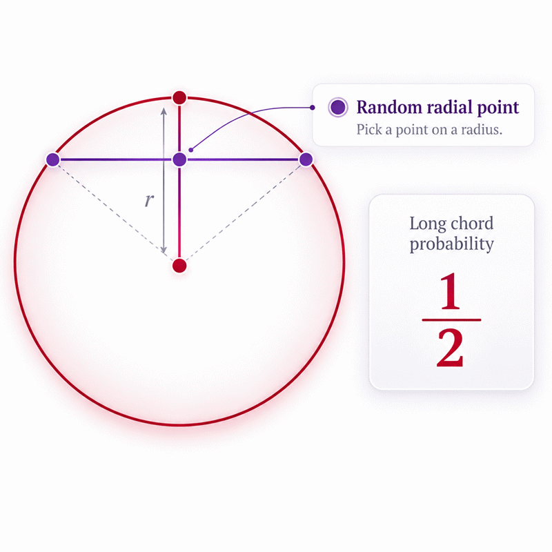
- Uniform radial midpoint distance produces the classic one-half probability.
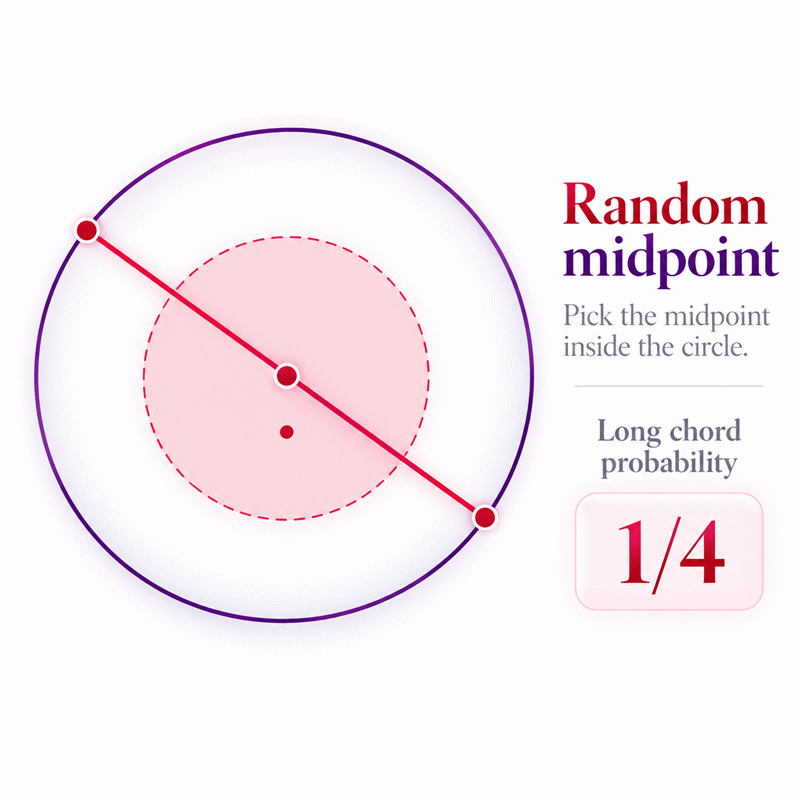
- Uniform midpoint sampling across disk area produces the classic one-quarter probability.
- The geometry stays unchanged while the probability measure changes.
- A custom chord threshold can be evaluated under all three standard models.
- Reverse solving can recover a compatible radius or chord threshold.
- The selected sampling model must remain consistent during reverse calculation.
- Monte Carlo results should approach the theoretical value for their own sampling procedure.
The Bertrand’s Paradox Calculator is most useful when you first identify how the chord is generated. It then lets you compare the same geometry under multiple probability models instead of treating the word random as a complete mathematical definition. This approach makes the paradox easier to understand and helps prevent the same sampling mistake in broader statistical work.
Assumptions used in this calculator
- The selected sampling method defines the probability model used.
- Random chords are not assumed to have one universal distribution.
- Circle geometry is treated as ideal and perfectly continuous.
- The circle radius must be positive and finite.
- Custom chord thresholds cannot exceed the circle diameter.
- Probability inputs use decimal or percent units consistently.
- Length inputs are converted to meters before calculation.
- Unit conversion does not change the underlying physical length.
- Intermediate calculations retain full JavaScript numeric precision.
- Displayed results may be rounded without changing stored values.
- Reverse solutions follow the same selected sampling model.
- Boundary probabilities depend on the strict longer-than comparison.
- Physical experiments may differ from ideal theoretical sampling.
Results are rounded for display.
Internal calculations use full precision.
Formulas Used in Bertrand's Paradox Variables and Calculation :
Length Unit Normalization
Probability Unit Normalization
Classic Equilateral-Triangle Threshold
Normalized Chord Threshold Ratio
Critical Midpoint Distance
Random Endpoints Probability
Random Radial-Point Probability
Random Midpoint Probability
Reverse Threshold from Endpoints Probability
Reverse Threshold from Radial Probability
Reverse Threshold from Midpoint Probability
Reverse Radius from Endpoints Probability
Reverse Radius from Radial Probability
Reverse Radius from Midpoint Probability
- R
- Circle radius in meters after unit conversion.
- L
- Chord-length threshold in meters after unit conversion.
- x
- Dimensionless ratio of the threshold to the circle diameter.
- Dc
- Maximum midpoint distance that produces a chord longer than L.
- P
- Decimal probability used by the selected sampling method.
- Pendpoints
- Probability calculated using random endpoints.
- Pradial
- Probability calculated using a uniformly selected radial midpoint distance.
- Pmidpoint
- Probability calculated using a uniformly selected midpoint in the disk.
- Vu
- Length value displayed in the selected user unit.
- Vm
- Equivalent length value converted to meters.
- fu
- Selected length-unit conversion factor to meters.
- Pu
- Probability value displayed in percent or decimal form.
- fp
- Probability conversion factor, 0.01 for percent and 1 for decimal.
Variables & Definitions
View a complete list of all variables used in this calculator, including definitions and units
Bertrand's Paradox Variables and Calculation Symbols
| Variable | Meaning | Base Unit | Role | Valid Domain |
|---|---|---|---|---|
| R | Circle radius | m | Input or reverse-solved value | R > 0 |
| L | Chord-length threshold | m | Input or reverse-solved value | 0 <= L <= 2R |
| x | Normalized threshold ratio | Dimensionless | Derived calculation variable | 0 <= x <= 1 |
| P | Probability for the selected sampling method | Decimal | Input or calculated value | 0 <= P <= 1 |
| P% | Probability expressed as a percentage | % | User-facing probability representation | 0% to 100% |
| P_endpoints | Probability under random endpoint sampling | Decimal | Calculated comparison result | 0 to 1 |
| P_radial | Probability under random radial-point sampling | Decimal | Calculated comparison result | 0 to 1 |
| P_midpoint | Probability under random midpoint sampling | Decimal | Calculated comparison result | 0 to 1 |
| D_c | Maximum midpoint distance for a chord longer than L | m | Derived geometric value | 0 to R |
| V_u | Displayed length value in the selected unit | Selected length unit | Unit conversion source | Finite numeric value |
| V_m | Equivalent internal length value in meters | m | Base-unit calculation value | Finite numeric value |
| f_u | Conversion factor from the selected length unit to meters | Dimensionless | Unit conversion factor | Positive constant |
| P_u | Displayed probability value in the selected probability unit | % or decimal | Probability unit conversion source | Unit-dependent |
| f_p | Conversion factor from the selected probability unit to decimal | Dimensionless | Probability conversion factor | 0.01 or 1 |
Unit Conversion Table
Length Unit Conversion Table for Radius and Chord Threshold
| Unit Group | Unit Name | Symbol | Equivalent in Meters | Used For |
|---|---|---|---|---|
| Popular Units | Meter | m | 1 m | Circle radius and chord threshold |
| Popular Units | Centimeter | cm | 0.01 m | Circle radius and chord threshold |
| Popular Units | Millimeter | mm | 0.001 m | Circle radius and chord threshold |
| Popular Units | Kilometer | km | 1000 m | Circle radius and chord threshold |
| Popular Units | Inch | in | 0.0254 m | Circle radius and chord threshold |
| Popular Units | Foot | ft | 0.3048 m | Circle radius and chord threshold |
| Popular Units | Yard | yd | 0.9144 m | Circle radius and chord threshold |
| Popular Units | Mile | mi | 1609.344 m | Circle radius and chord threshold |
| Scientific Units | Micrometer | um | 0.000001 m | Circle radius and chord threshold |
| Scientific Units | Nanometer | nm | 0.000000001 m | Circle radius and chord threshold |
Probability Unit Conversion Table
| Unit Group | Unit Name | Symbol | Equivalent in Decimal Probability | Used For |
|---|---|---|---|---|
| Popular Units | Percent | % | 1% = 0.01 | Probability input and result display |
| Scientific Units | Decimal Probability | decimal | 1 decimal = 1 | Probability input and internal probability scale |
Example Calculation
The threshold is 75% of the circle diameter.
Random endpoint sampling gives a 46.01069123% longer-chord probability.
The same geometry produces different probabilities under different sampling models.
Intermediate values remain unrounded; formatting occurs only at display time.
The probability is first converted from 64% to 0.64.
The midpoint inverse equation then solves the missing circle radius.
A 6 m threshold and 64% probability require a 5 m radius.
The resolved geometry is then reused for all three comparison probabilities.
Results are rounded for display.
Internal calculations use full precision.
Calculations Disclaimer
Why Can One Random Chord Problem Have Three Correct Answers?
A simple probability question can fail before any arithmetic begins. Bertrand’s Paradox Calculator exposes that failure immediately. Bertrand’s Paradox Calculator does not ask users to accept one mysterious answer. It shows why the meaning of random must be fixed first.
Imagine the same circle throughout the entire problem. The geometry never changes. The threshold can also stay unchanged. Yet three standard sampling procedures produce different probabilities. That seems impossible at first. It becomes clear once the random experiment is defined.
A probability does not belong to an object alone. It belongs to a model of how outcomes occur. A circle contains infinitely many possible chords. Saying that one chord is chosen randomly does not state how those chords receive probability weight.
The standard endpoint model produces one result. A radial selection model produces another. Uniform midpoint sampling over the disk produces a third. None requires the circle to change.
What the Word Random Changes Before Any Probability Is Calculated
The practical problem is hidden inside one word: random. Suppose a user says points are selected uniformly. The next question must be, “uniformly over what?” Equal angle intervals, equal radial intervals, and equal areas describe different distributions.
This matters far beyond a classroom paradox. Analysts face the same issue with real data. A sample can appear unbiased while its selection rule favors certain outcomes. A clear sampling mechanism prevents that mistake.
AxiCalculator therefore keeps the three chord models separate. The user chooses a model rather than receiving an unexplained probability. That choice is part of the calculation itself.
Why Equal-Looking Sampling Rules Do Not Create Equal Distributions
Two selection rules may both look fair. They can still weight the same geometry differently. Uniform distance from the center does not produce uniform area across a disk. Outer rings contain more area than inner rings.
Likewise, choosing two endpoints uniformly does not create the same midpoint distribution. This is the central lesson. Uniformity depends on the variable being sampled.
Random radial point → center distance receives equal weight → another chord distribution
Random midpoint → disk area receives equal weight → a third chord distribution
How Random Endpoints Produce the One-Third Result
A user may expect every construction to produce the same answer. The endpoint model shows why that expectation fails. Here, a chord is determined from two positions on the circumference.
Rotational symmetry allows one endpoint to be treated as fixed. The second endpoint then moves around the circle. Only a certain opposite arc creates a chord longer than the classic triangle side. That favorable arc occupies one third of the full circumference.
The resulting probability is therefore one third. It is not an approximation caused by a calculator. It belongs to the endpoint sampling process itself.
The Geometry Behind the Qualifying Arc
The geometry becomes easier when the inscribed triangle is mentally rotated. One vertex can align with the fixed chord endpoint. The other two vertices identify the relevant opposite arc.
When the second endpoint falls inside that arc, the chord exceeds the triangle side. Outside it, the chord becomes shorter. The event is therefore measured by an angular fraction.
This construction is especially useful when the physical or simulated experiment truly selects circumference endpoints independently.
When the Random Endpoints Model Matches Your Experiment
Use this model only when the actual mechanism matches endpoint sampling. A simulation might independently choose two angles around a circle. That process naturally fits the endpoint interpretation.
Do not select this method merely because one third looks familiar. The procedure determines the model. The expected number is a consequence.
How Random Radial Points Produce the One-Half Result
Another user may generate chords from their distance to the center. The answer now changes. A radius direction is chosen, then a position is selected uniformly along that radius. A perpendicular chord passes through that position.
Longer chords pass nearer the center. Shorter chords sit closer to the boundary. In the classic triangle setup, the critical position lies halfway along the radius.
Half of the uniformly sampled radial distance lies on the qualifying side. The resulting probability becomes one half.
Why Midpoint Distance Controls Chord Length
A chord expands as its midpoint moves toward the circle center. At the center, the chord becomes a diameter. Moving outward shortens it continuously.
This relationship converts a length question into a distance question. Instead of testing chord length directly, the model can test whether the chord midpoint lies within a critical center distance.
That geometric transformation is also useful for generalized thresholds. It lets the calculator compare the same geometry under several probability measures.
Why Uniform Radius Is Different from Uniform Area
This distinction causes many wrong explanations. A radial interval and a disk region are not the same type of sample space.
Equal steps along a radius give every distance interval equal weight. Uniform area sampling gives larger outer rings more weight because they contain more area.
The circle has not changed. Only the distribution of midpoint locations has changed.
How Random Midpoints Produce the One-Quarter Result
A third experiment selects the chord midpoint uniformly across the disk. The user may assume this resembles uniform radial distance. It does not.
For the classic threshold, qualifying midpoints lie within a smaller concentric region. That region has half the original radius. Area scales with the square of radius.
The favorable region therefore occupies one quarter of the disk. The probability becomes one quarter.
The Area Logic Behind the Midpoint Method
Think in regions rather than line segments. Every equal patch of disk area has equal chance of containing the chosen midpoint.
The inner qualifying disk is smaller in both width and height. Halving its radius reduces its area much more sharply. That geometric fact produces the quarter result.
This method is appropriate when points are genuinely generated uniformly over disk area.
Why Midpoint Density Changes as Distance Increases
Equal radial bands do not contain equal area. A thin band near the outer boundary covers much more space. That means uniform area sampling naturally produces more midpoint locations at larger radii.
This is why a uniformly selected disk midpoint cannot be modeled as a uniformly selected radial distance. Confusing those two procedures swaps one half and one quarter.
Change endpoint weighting → probability changes
Change radial-distance weighting → probability changes
Change area weighting → probability changes
The difference is the probability measure, not the geometry.
How Should You Choose the Correct Bertrand Sampling Method?
The most important practical decision is not numerical. It is experimental. Ask exactly how the chord is generated.
If two circumference locations are selected independently, use the endpoint model. If the midpoint distance along a radius is uniform, use the radial model. If the midpoint itself is uniform over disk area, use the midpoint model.
The calculator makes these models explicit. This avoids a common failure: calculating correctly from the wrong assumptions.
Match the Probability Model to the Actual Random Experiment
Real experiments often contain details absent from textbook wording. A physical line may have finite length. A simulation may reject lines that miss the circle. A data generator may sample coordinates rather than radial distances.
Those details matter. They can alter the induced chord distribution. A label such as “random” cannot replace a description of the process.
For professional analysis, document the generator before reporting its probability.
How Reverse Solving Changes the Question Without Changing the Model
Sometimes the probability is known while a geometric quantity is missing. Reverse solving can recover a compatible radius or threshold.
The critical rule is consistency. The same sampling model must remain selected. A probability generated under endpoint sampling cannot be inverted using midpoint assumptions.
AxiCalculator keeps that relationship visible. Editable results can become known values while another variable becomes the unknown.
What Does the Invariance View Add to Bertrand’s Paradox?
A physical experiment creates another layer of difficulty. How should an apparently random line arrive at the circle? Where is the circle placed? Does changing its scale alter the rule?
An invariance approach asks whether the process remains consistent under transformations. This can be valuable when defining a physical random-line experiment.
However, this does not make every other mathematical measure disappear. Those measures still describe different well-defined experiments.
Why Physical Random-Line Experiments Need More Information
A real object cannot behave like an infinitely long mathematical line automatically. Its length, placement, orientation, and acceptance rules may influence which chords are retained.
That difference explains why experimental observations may diverge from a simple classroom result. Before comparing theory with measurements, reproduce the experimental protocol carefully.
Why One Physical Model Does Not Erase Other Probability Measures
A useful physical construction can answer a specific operational question. It does not prove that endpoint or midpoint models are algebraically invalid.
Each model describes a different probability space. The safer language is therefore precise: identify the selected measure and report its result.
How Can Monte Carlo Simulation Check Each Chord Model?
Simulation often creates a new problem. Users run thousands of trials and expect an exact theoretical percentage. Finite simulations rarely produce it exactly.
A Monte Carlo experiment repeatedly generates chords using one rule. The observed success rate should move near that model’s theoretical probability as trials grow.
The simulation checks implementation and intuition. It does not decide which sampling rule nature must use.
Why Different Simulations Converge to Different Limits
If two programs generate chords differently, their results can stabilize around different values. That is expected here.
A program choosing random circumference endpoints should approach the endpoint result. Uniform radial distance should approach the radial result. Uniform disk midpoints should approach the midpoint result.
Different convergence targets therefore reveal different probability models, not broken mathematics.
How Trial Count Changes Noise but Not the Underlying Model
Increasing trials reduces random fluctuation. It does not repair a poorly specified model.
One million trials of the wrong sampling process only estimate that wrong process more precisely. Model definition must come before sample size.
Which Common Mistakes Change the Bertrand’s Paradox Answer?
The most damaging mistake is treating “random” as a complete mathematical instruction. It is not. Another error is mixing a uniform radius with uniform area.
Users also switch models during reverse solving. Some compare simulated results generated by one rule against theoretical values from another. Others interpret finite Monte Carlo noise as evidence against theory.
A less obvious mistake involves the comparison threshold. Changing the target chord length changes the probability even when the sampling model stays fixed.
How to Audit the Sampling Rule Before Trusting the Result
Start with three questions. What object is sampled? Which variable is uniform? What event counts as success?
Next, check whether the physical or simulated procedure matches those statements. Only then compare the final probability.
This audit takes seconds. It prevents a large class of statistical mistakes.
What Does Bertrand’s Paradox Teach Us About Probability Models?
Bertrand’s paradox teaches a broader lesson than any single fraction. Probability requires a sample space and a measure. Geometry alone does not decide how outcomes receive probability.
This insight transfers directly to data science, engineering simulation, reliability studies, and experimental statistics. Sampling procedures shape observed distributions. Hidden selection rules can shape conclusions.
AxiCalculator makes that dependency visible. Users can compare standard models, change the geometric threshold, and reverse-solve compatible quantities. The goal is not to force one answer. The goal is to make every answer traceable to its assumptions.
That is the practical value of the paradox. It trains a habit worth keeping: never ask only for the probability. Ask how the outcomes were generated.
Frequently Asked Questions
Does changing the circle radius change the classic Bertrand probabilities?
Can two people simulate Bertrand's paradox correctly and still get different results?
Why should I use a custom chord threshold instead of only the classic triangle side?
Can Bertrand's paradox help me understand real statistical sampling problems?
How should I validate a Monte Carlo implementation of the three chord models?
Can a physical line or straw experiment be treated as one of the ideal Bertrand models automatically?
Why must reverse solving preserve the selected sampling method?
Our engineers are here to help you get it right.