Parrondo’s Paradox Variables
- Last formula update:

Decimal & Rounding Policy
- Probabilities are calculated internally in decimal form without intermediate rounding.
- Decimal, percent, and basis-point inputs are converted before calculations begin.
- Displayed numerical results use up to six decimal places when needed.
- Trailing zeros may be omitted without changing the underlying calculated value.
- Strategy classification uses the unrounded expected net capital change.
- Values extremely close to zero are treated as fair only for classification stability.
Valid range
- Strategy: Game A, Game B, AB, AABB, or Random A/B with equal selection probability.
- Number of games: integer values from 1 to 5000.
- Initial capital: integer values from -1000000000 to 1000000000 units.
- Epsilon: 0 inclusive to 0.1 exclusive, with 0.005 as the default value.
- P(A): greater than 0.4 and up to 0.5 under the linked epsilon model.
- P(B1): greater than 0 and up to 0.1 under the linked epsilon model.
- P(B2): greater than 0.65 and up to 0.75 under the linked epsilon model.
- Decimal probability: values must remain between 0 and 1.
- Percent probability: values must remain between 0% and 100%.
- Basis-point probability: values must remain between 0 and 10000 bp.
- Reverse-entered probabilities must produce one valid shared epsilon value.

Wylena Brantford
Reviewers:
Valdren Clyforde
Zenara Dentwick
Check our editorial policy
September 19, 2026
1.0.0
Initial calculator and formula release.
Our engineers are here to help you get it right.
How Does Parrondo’s Paradox Calculator Reveal a Winning Combination?
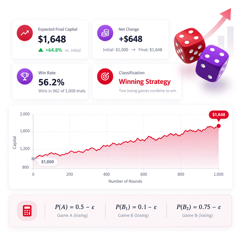
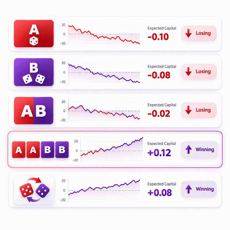
Parrondo’s Paradox Calculator shows how two individually losing games can create a positive expected outcome when switching changes the system’s state distribution. The calculator compares Game A, capital-dependent Game B, AB, AABB, and random A/B selection while tracking expected capital and the direction of the strategy.
- Game A uses a small fixed negative bias.
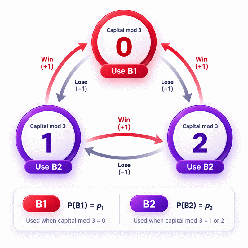
- Game B changes its winning probability according to capital modulo three.
- The unfavorable B1 branch applies when capital is divisible by three.
- The favorable B2 branch applies in the other two remainder states.
- Switching strategies can change how often those states occur.
- AABB and random mixing can therefore behave differently from either isolated game.
- Expected capital separates the mathematical trend from one lucky or unlucky random path.
- Changing epsilon updates the linked Game A, B1, and B2 probabilities together.
Use Parrondo’s Paradox Calculator to test one strategy at a time under identical parameters. Compare expected final capital, net change, win rate, and trajectory. The key lesson is simple: switching does more than average two games because it can reshape the states encountered by a state-dependent process.
Assumptions used in this calculator
- Each win changes capital by exactly plus one unit.
- Each loss changes capital by exactly minus one unit.
- Game A uses one fixed winning probability.
- Game B depends only on capital modulo three.
- Capital states are integers throughout every evaluated game.
- Epsilon links all three winning probabilities consistently.
- Random strategy selects Game A and Game B equally.
- AB strategy alternates one A game with one B game.
- AABB strategy repeats two A games followed by two B games.
- Exact expectation replaces finite Monte Carlo sampling noise.
- Probability values remain constant during a calculation.
- No transaction costs, stakes, fees, or external effects are modeled.
- Displayed rounding never changes internal calculation precision.
Results are rounded for display.
Internal calculations use full precision.
Formulas Used in Parrondo's Paradox Variables :
Linked Winning Probabilities
Capital-Dependent Game B Probability
Strategy Winning Probability
Probability Distribution Update
Expected Final Capital
Expected Net Change and Win Rate
Reverse Probability Calculation
Probability Unit Conversion
- ε: shared probability-bias parameter.
- pA: probability of winning Game A.
- pB1: Game B winning probability when capital is divisible by 3.
- pB2: Game B winning probability otherwise.
- c: a possible integer capital state.
- C0: initial capital.
- CN: capital after N games.
- n: zero-based game index.
- N: total number of evaluated games.
- Dn(c): probability of capital c after n games.
- pn(c): winning probability at turn n from capital c.
- Δ: expected net capital change.
- p̄: expected average winning probability.
- p: a generic decimal probability used for unit conversion.
Variables & Definitions
View a complete list of all variables used in this calculator, including definitions and units
Parrondo's Paradox Variables and Model Parameters
| Variable | Meaning | Definition or Role | Valid Range or Type |
|---|---|---|---|
| ε | Bias parameter | Links the three game-winning probabilities. | 0 ≤ ε < 0.1 |
| pA | Game A win probability | 0.5 − ε | 0.4 < pA ≤ 0.5 |
| pB1 | Game B1 win probability | Used when current capital is divisible by 3. | 0 < pB1 ≤ 0.1 |
| pB2 | Game B2 win probability | Used when current capital is not divisible by 3. | 0.65 < pB2 ≤ 0.75 |
| c | Capital state | A possible integer capital value during evaluation. | Integer |
| C0 | Initial capital | Capital before the first game. | -1000000000 to 1000000000 |
| CN | Final capital | Capital after N evaluated games. | Integer state variable |
| n | Game index | Identifies the current step in a strategy sequence. | 0 to N − 1 |
| N | Number of games | Total number of evaluated game steps. | Integer from 1 to 5000 |
| Dn(c) | Capital probability distribution | Probability of occupying capital state c after n games. | 0 to 1 |
| pn(c) | Turn-specific win probability | Winning probability selected by strategy and capital state. | 0 to 1 |
| E[CN] | Expected final capital | Probability-weighted mean capital after N games. | Real number |
| Δ | Expected net change | Expected final capital minus initial capital. | Real number |
| p̄ | Expected average win rate | Average implied winning probability across all evaluated games. | 0 to 1 |
| p | Generic probability | Decimal probability used for display-unit conversion. | 0 to 1 |
Unit Conversion Table
Parrondo's Paradox Probability Unit Conversion Table
| Unit Group | Unit Name | Symbol | Equivalent in Decimal | Used For |
|---|---|---|---|---|
| Probability | Decimal Probability | p | 1 = 1.0000 | Internal probability calculations for epsilon, P(A), P(B1), and P(B2) |
| Probability | Percent | % | 1% = 0.01 | User-friendly probability entry and display |
| Probability | Basis Point | bp | 1 bp = 0.0001 | Fine-grained probability values and small epsilon differences |
Example Calculation
The AABB sequence uses the linked probabilities without rounding intermediate values. The exact capital distribution is propagated through all 100 game steps. Its expected final capital is above the starting capital, producing a positive net change. The result therefore classifies this parameter set and sequence as winning.
The reverse calculation starts from the editable P(B2) value. Subtracting that probability from 0.75 recovers the shared epsilon. The recovered epsilon then determines P(A) and P(B1) automatically. Recalculating P(B2) confirms the entered value and verifies consistency.
Results are rounded for display.
Internal calculations use full precision.
Calculations Disclaimer
What Makes Parrondo’s Paradox Calculator Useful When Two Losing Games Mislead You?
A common problem appears when two losing games are judged separately. Parrondo’s Paradox Calculator exposes why that shortcut can fail. Parrondo’s Paradox Calculator also shows what changes after switching begins. The key is not magical probability. The key is the changing state of the system.
Game A has a small negative bias. Game B also loses under its own long-run state pattern. That sounds conclusive. Combining them should appear even worse. Yet certain switching rules can alter which Game B states occur most often. That change can reverse the expected direction.
Why Looking at Each Game Alone Creates the Wrong Intuition
The first problem is simple averaging. People often imagine two negative expectations being averaged together. That reasoning assumes the underlying situations remain unchanged. They do not remain unchanged here.
Game B reacts to current capital. A previous result can therefore change the next probability. Switching games changes capital before Game B returns. That means switching also changes future exposure to Game B’s branches.
This is why the paradox becomes easier after one mental shift. Stop asking only which game has better odds. Ask which states each strategy creates.
What Changes When the Games Share a Capital State
The next problem is hidden dependence. Game A does not inspect capital before choosing its odds. Game B does. Both games still modify the same capital.
That shared capital becomes a bridge between them. A result from Game A can move capital into another remainder class. Game B then reacts to that new class. The next probability is therefore influenced indirectly by the previous game.
Eye-drag insight: Losing game → state shift → different branch → changed long-run exposure.
That sequence explains more than the word “paradox.” It tells you exactly what to inspect. A good calculator should reveal strategy, expected capital, net change, and trajectory together. AxiCalculator is designed around that decision path.
How Does Game A Create a Small but Persistent Losing Drift?
A real analysis problem starts with a nearly fair game. A tiny bias can look harmless over ten rounds. It becomes meaningful across many rounds.
In the standard setup, Game A wins slightly less than half the time. A win adds one capital unit. A loss removes one capital unit. The two outcomes have equal size. Their probabilities are not equal.
That imbalance creates a negative expected movement. It is small per turn. Repetition makes it visible.
Why a 49.5 Percent Win Chance Matters Over Many Games
The common mistake is focusing on 49.5 percent as “almost fifty-fifty.” That description is psychologically reasonable. It is mathematically incomplete.
A symmetric gain and loss needs a fifty percent win chance for fairness. Any persistent shortfall creates negative drift. The effect may be hidden by randomness during short runs. Expected behavior still points downward.
This distinction matters when comparing strategies. A single lucky path does not turn Game A into a winning process. A single unlucky path also does not measure its expectation.
What a Small Negative Bias Does to Expected Capital
The practical problem is separating noise from direction. A random sample can move upward temporarily. Expected capital asks a different question. It averages the possible outcomes according to their probabilities.
This is why exact expectation is valuable in an educational calculator. The same inputs always return the same expected result. Users can then compare strategies without a lucky random seed changing the story.
Text infographic:
Nearly fair coin → slight negative bias → repeated exposure → negative expected drift.
Use that chain as the baseline. The paradox becomes meaningful only after both component strategies are understood correctly.
Why Can Game B Lose Even With a Strong 74.5 Percent Coin?
The confusing problem appears immediately. Game B contains a coin that wins far more than half the time. Many users therefore expect Game B to be profitable.
That conclusion ignores when the favorable coin is selected. Game B is not one fixed coin. It is a state-dependent rule.
When capital belongs to the unfavorable remainder class, Game B uses B1. Otherwise, it uses B2. The important question is therefore not only the probability of B2. The important question is how often each branch gets used.
How Capital Modulo Three Chooses Between B1 and B2
The next problem is understanding the state test. Capital is divided conceptually into three remainder classes. These classes repeat across every integer capital value.
One class triggers the unfavorable B1 coin. The other two trigger B2. This might suggest B2 should dominate automatically. State movement prevents that simple conclusion.
Wins and losses shift capital by one unit. Those moves also shift the remainder class. The process therefore creates its own pattern of future states.
Watch this shift: capital → remainder class → Game B branch → next capital.
Why the Bad State Appears Often Enough to Matter
The hidden problem is state occupancy. Three remainder classes do not have to occur equally often. Transition probabilities decide their long-run frequencies.
Game B can steer the process toward a distribution where the unfavorable branch appears often enough. Its severe disadvantage can then offset the strong B2 probability.
This is the point where intuition often breaks. The favorable coin is genuinely favorable. Game B can still lose as a whole.
The lesson extends beyond this calculator. Conditional probabilities should never be judged without their exposure frequencies. AxiCalculator makes this easier by keeping the strategy result and capital behavior visible together.
How Can Switching Between Losing Games Reverse the Direction?
The real puzzle begins after both isolated games are understood. If A loses and B loses, why can switching produce growth?
Switching changes the state distribution before Game B acts again. That is the mechanism. No probability law is broken. No hidden profit appears from nowhere.
A strategy such as AABB inserts Game A at specific positions. Those plays alter capital without using Game B’s state rule. When B returns, it can encounter a different mix of remainder states.
Why AABB Reshapes the States Seen by Game B
The practical problem is sequence timing. Two A plays can move capital through remainder classes before two B plays arrive.
The B games therefore do not face the same state distribution produced by continuous B play. Their branch exposure changes. That can reduce the long-run influence of the unfavorable B1 state.
This is why AABB should not be described as simple averaging. The order itself affects the environment seen by later turns.
How Random Mixing Changes Long-Run State Exposure
Another problem appears when switching is random. Random does not mean irrelevant. Choosing A or B with equal probability still changes state transitions.
Whenever A is chosen, it modifies capital using its fixed probability. Whenever B returns, it responds to the resulting state. Repeating that interaction can create a new long-run distribution.
The compound process therefore deserves its own analysis. It is not merely half of A plus half of B.
Why Combining Expectations Is Not the Same as Combining States
The common error is adding two isolated averages. That ignores the fact that Game B’s average changes with state occupancy.
Text infographic:
Play A or B → capital moves → state mix changes → B branch frequency changes → expected drift changes.
This is the shortest useful explanation of the paradox. The combined strategy changes the conditions under which one component operates.
How Does Markov Thinking Resolve Parrondo’s Paradox?
The technical problem is explaining the result without relying on surprise. Markov thinking provides a clean solution.
You do not need advanced theory to understand the core idea. Group capital by its remainder after division by three. The system then has three repeating state classes.
A win moves the process forward one class. A loss moves it backward one class. The transition probability depends on the selected game and current state.
What the Three Capital Remainder States Reveal
The first Markov problem is identifying enough information about the present. Exact capital may be large or negative. Game B only needs its remainder class.
That reduces an infinite set of possible capital values into three repeating categories for branch selection. State zero uses the unfavorable branch. The other two use the favorable branch.
Once transitions between these categories are tracked, the apparent contradiction disappears. Different strategies create different transition patterns.
Why Stationary State Occupancy Matters More Than One Coin Toss
The next problem is judging a process from individual turns. One toss says almost nothing about long-run branch exposure.
Long-run state occupancy describes where the process spends its time. If a strategy changes that occupancy, it changes the average probability experienced during Game B.
This is why a trajectory chart is useful. It provides a visual check on expected direction. It should not replace the state logic. It should confirm it.
Eye-drag insight: The coin probabilities stay fixed. The frequency of seeing them changes.
That single distinction resolves most confusion surrounding Parrondo’s paradox.
Which Parrondo Strategy Should You Test First?
The practical problem is choosing a strategy without creating a misleading comparison. Start every comparison with identical parameters.
Keep epsilon unchanged. Keep the number of games unchanged. Keep initial capital unchanged. Then change only the strategy.
This creates a clean experiment. Game A provides the fixed-bias baseline. Game B shows the state-dependent baseline. Alternating strategies reveal what switching changes.
Game A vs Game B vs AB vs AABB vs Random Mixing
The first decision problem is understanding what each option tests. Game A isolates fixed negative bias. Game B isolates the capital-dependent mechanism.
AB forces strict one-for-one alternation. AABB creates a four-turn repeating block. Random mixing makes a fresh A-or-B selection every turn.
These are not interchangeable labels. Each strategy produces its own transition sequence. That sequence can create a different expected capital path.
A useful comparison focuses on expected final capital and net change. Win rate adds supporting context. Strategy classification provides a quick summary.
Why the Best Pattern Depends on the Parameters
The next problem is assuming one pattern must always win. That is unsafe. Parrondo behavior depends on the probabilities and switching rules.
A pattern that works under the standard setup can behave differently after parameters change. Epsilon shifts all three linked probabilities. That can weaken or remove the positive compound effect.
This is why interactive testing matters. Change one factor at a time. Watch whether the expected trajectory remains positive.
Use AxiCalculator as an analysis tool, not as a promise that a named sequence always wins.
What Can Make a Parrondo Calculation Misleading?
The biggest real problem is confusing a random result with mathematical expectation. A short simulation can move in the wrong direction by chance.
Another problem is changing several parameters at once. That makes the cause of a result difficult to identify. A third problem is breaking the linked probability model accidentally.
Good analysis keeps the model coherent. It also distinguishes expected results from individual random paths.
Why One Short Random Simulation Can Give the Wrong Impression
The sampling problem is strongest when the expected effect is small. Random wins and losses can overwhelm the drift over a short horizon.
A winning expected strategy may finish below zero in one sample. A losing strategy may finish above zero. Neither outcome changes the underlying expectation.
Exact expectation avoids this specific source of noise. It propagates probability across all reachable outcomes instead of selecting one random path.
That makes repeated comparisons reproducible. It is especially useful for teaching and QA.
Why State Rules Must Stay Consistent Across Every Turn
The implementation problem is easy to underestimate. Game B must inspect current capital before every B turn.
Using the previous capital incorrectly changes the process. Applying B1 to the wrong remainder class also changes the model. Rounding probabilities during intermediate steps can create further drift.
Eye-drag check: same rules, same inputs, same expected result.
A reliable implementation should therefore preserve full internal precision. It should also validate linked parameters before evaluating a strategy.
How Should You Use Parrondo’s Paradox Calculator for Study and Analysis?
The final practical problem is turning an interesting paradox into a useful learning workflow. Random clicking teaches very little.
Begin with the standard setup. Compare Game A and Game B first. Confirm that both expected trajectories are negative. Then test AABB and random mixing.
After the mechanism becomes clear, change one parameter. Observe how the direction changes. Repeat with a different starting capital or game count.
A Faster Workflow for Students, Teachers, and Probability Researchers
The student problem is often conceptual. Start by predicting the result before calculating. Then compare your prediction with the output.
The teaching problem is usually visibility. Use the trajectory and strategy comparison to show that switching changes state exposure. Ask students to explain the change before introducing formal Markov notation.
The research problem is reproducibility. Keep parameters fixed, record the strategy, and compare exact expected values under identical conditions.
AxiCalculator makes that workflow faster because the model updates immediately. You can also reverse-solve linked probability inputs. This helps test whether different representations describe the same epsilon.
The most useful conclusion is not “two losses magically create a win.” A better conclusion is more precise. State-dependent processes can change when their dynamics are switched. That is the real insight behind Parrondo’s paradox.
Run several strategies, compare their trajectories, and challenge your first intuition. The value of this calculator is not only the final number. It is seeing exactly which assumption made the direction change.
Frequently Asked Questions
Can a positive expected Parrondo strategy still finish with a loss?
Does changing the starting capital change which Game B coin is used first?
Why should I compare strategies with identical epsilon and game counts?
Can Parrondo's paradox be treated as a guaranteed money-making method?
How can an engineer verify that a Parrondo implementation uses the correct state timing?
Why can direct expected-value averaging give the wrong compound-game conclusion?
How should a researcher compare exact expectation with Monte Carlo output?
Engineering Resources
Our engineers are here to help you get it right.