Relative Risk Calculator
- Last formula update:

Decimal & Rounding Policy
- Keep full floating-point precision throughout all relative risk and confidence interval calculations.
- Never round group risks, logarithms, standard errors, Z-scores, or bounds during intermediate calculations.
- Display final finite results with up to 12 significant digits and remove unnecessary trailing zeros.
- Preserve entered count precision, including valid decimal values produced by reverse solving.
- Do not force reverse-solved values to whole numbers unless the user explicitly changes them.
- Use scientific notation only when a result is too small or large for compact decimal display.
Valid range
- Confidence level: greater than 0% and less than 100%; supported range is 0.000001% to 99.999999%.
- Z-score: finite, greater than 0, and no greater than 8.2095361516.
- Exposed disease count (a): greater than 0 and no greater than 1e15 for log-based confidence intervals.
- Exposed no-disease count (b): finite, nonnegative, and no greater than 1e15.
- Control disease count (c): greater than 0 and no greater than 1e15 for log-based confidence intervals.
- Control no-disease count (d): finite, nonnegative, and no greater than 1e15.
- Exposed group total: a + b must be greater than 0.
- Control group total: c + d must be greater than 0.
- Relative risk: finite and greater than 0 whenever supplied as a reverse-solving input.
- Lower confidence bound: finite, greater than 0, and below RR when solving confidence inversely.
- Upper confidence bound: finite, greater than 0, and above RR when solving confidence inversely.
- Reverse-solved counts must remain finite, nonnegative, and within the supported count range.

Wylena Brantford
Reviewers:
Valdren Clyforde
Zenara Dentwick
Check our editorial policy
September 14, 2026
1.0.0
Initial calculator and formula release.
Our engineers are here to help you get it right.
What Does a Relative Risk Calculator Tell You About Two Groups?
Relative Risk Calculator results show how the observed probability of an outcome in one group compares with the probability in a reference group. The result is expressed as a unitless risk ratio, making direction easy to read while keeping the original study context important.
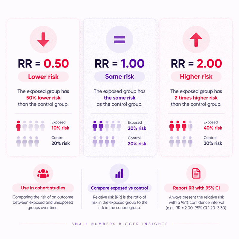
- RR = 1 means the observed risks are equal.
- RR > 1 means the numerator group has higher observed risk.
- RR < 1 means the numerator group has lower observed risk.
- The confidence interval shows the statistical precision of the estimate.
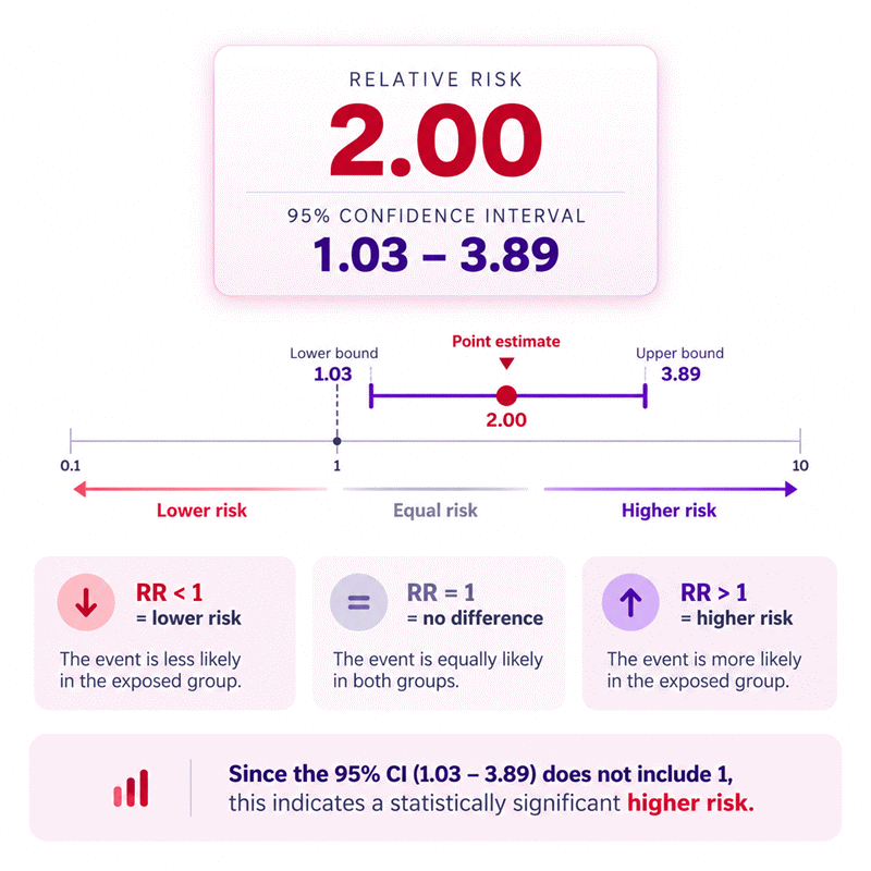
- An interval containing 1 remains compatible with the null value.
- Relative risk does not establish causation by itself.
- Cohort studies and randomized trials commonly support direct risk comparison.
- Traditional case-control studies generally require an odds-ratio approach instead.
- Baseline risk should be checked before judging practical importance.
- Reverse solving can reconstruct one missing value when enough information exists.
The AxiCalculator Relative Risk Calculator helps organize exposed and control data, compare event risk, inspect statistical uncertainty, and test compatible reverse-solving scenarios. Always interpret the output together with study design, data quality, sample information, potential bias, and the real-world importance of the outcome.
Assumptions used in this calculator
- Exposed and control groups are defined consistently and independently.
- Each participant contributes to one group and one outcome category.
- Disease status is binary and measured consistently across both groups.
- Counts represent the same observation period and target population definition.
- Relative risk compares exposed risk directly with control group risk.
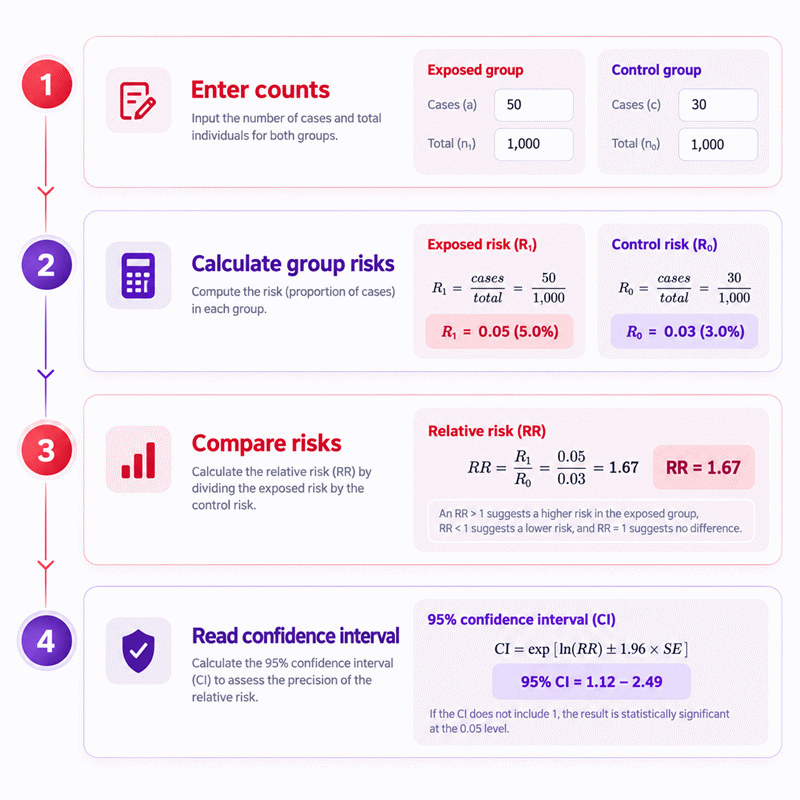
- Confidence intervals use the logarithmic large-sample approximation for relative risk.
- Disease counts in both groups are positive for log-based intervals.
- No continuity correction is applied automatically to zero event cells.
- Confidence level represents a two-sided interval around the estimated relative risk.
- The selected Z-score corresponds to the chosen two-sided confidence level.
- Input values are finite, nonnegative, and internally consistent with group totals.
- Reverse-solved values satisfy the same relative-risk equation as forward calculations.
- Results describe association and do not establish causation or individual risk.
Results are rounded for display.
Internal calculations use full precision.
Formulas Used in Relative Risk Calculator :
Confidence Percentage Conversion
Bidirectional Confidence Level and Z-Score Mapping
Relative Risk
Standard Error of the Log Relative Risk
Confidence Interval Bounds
- C%
- Confidence level expressed as a percentage in the calculator interface.
- C
- Confidence level expressed as a decimal probability between 0 and 1.
- Zc
- Critical Z-score corresponding to the selected two-sided confidence level.
- a
- Number of exposed-group members who developed the disease.
- b
- Number of exposed-group members who did not develop the disease.
- c
- Number of control-group members who developed the disease.
- d
- Number of control-group members who did not develop the disease.
- RR
- Relative risk comparing exposed-group risk with control-group risk.
- SEln(RR)
- Standard error of the natural logarithm of relative risk.
- L
- Lower confidence bound for relative risk.
- U
- Upper confidence bound for relative risk.
- Φ
- Standard normal cumulative distribution function.
Reverse count solving uses algebraic isolation of the same relative-risk identity, so no additional statistical model is introduced.
Variables & Definitions
View a complete list of all variables used in this calculator, including definitions and units
Relative Risk Calculator Variables and Statistical Parameters
| Symbol | Variable | Meaning | Valid Range | Unit or Scale | Calculation Role |
|---|---|---|---|---|---|
| C% | Confidence level | Selected two-sided confidence level shown to the user. | 0.000001% < C% < 99.999999% | % | Determines the critical Z-score. |
| C | Decimal confidence probability | Confidence level converted from percent to decimal form. | 0 < C < 1 | Unitless | Input to the standard normal mapping. |
| Zc | Critical Z-score | Standard normal critical value for the selected confidence level. | 0 < Zc ≤ 8.2095361516 | Unitless | Controls confidence interval width. |
| a | Exposed disease count | Exposed-group members who developed the disease. | 0 < a ≤ 1e15 | Count | Defines exposed risk and log-RR variance. |
| b | Exposed no-disease count | Exposed-group members who did not develop the disease. | 0 ≤ b ≤ 1e15 | Count | Completes the exposed-group denominator. |
| c | Control disease count | Control-group members who developed the disease. | 0 < c ≤ 1e15 | Count | Defines control risk and log-RR variance. |
| d | Control no-disease count | Control-group members who did not develop the disease. | 0 ≤ d ≤ 1e15 | Count | Completes the control-group denominator. |
| RR | Relative risk | Ratio of exposed-group disease risk to control-group disease risk. | RR > 0 | Unitless ratio | Main calculator result and reverse-solving target. |
| SEln(RR) | Log relative risk standard error | Estimated uncertainty of the natural logarithm of RR. | SEln(RR) ≥ 0 | Unitless | Determines confidence interval spread. |
| L | Lower confidence bound | Lower endpoint of the confidence interval for RR. | L > 0 | Unitless ratio | Lower uncertainty limit. |
| U | Upper confidence bound | Upper endpoint of the confidence interval for RR. | U > 0 | Unitless ratio | Upper uncertainty limit. |
Unit Conversion Table
Confidence Level Scale Conversion
| Unit Group | Unit Name | Symbol | Equivalent in Decimal Probability | Used For |
|---|---|---|---|---|
| Probability Scale | Percent | % | 1% = 0.01 | Confidence level entry and display |
| Probability Scale | Decimal probability | 1 | 1.00 = 100% | Internal confidence calculation |
Dimensionless Statistical Measures
| Unit Group | Unit Name | Symbol | Equivalent in Unitless Form | Used For |
|---|---|---|---|---|
| Dimensionless Statistic | Z-score | Zc | 1 Z-score = 1 | Confidence interval critical value |
| Dimensionless Statistic | Relative risk | RR | 1 RR = 1 | Comparing exposed and control risks |
| Dimensionless Statistic | Lower confidence bound | L | 1 L = 1 | Lower relative risk interval limit |
| Dimensionless Statistic | Upper confidence bound | U | 1 U = 1 | Upper relative risk interval limit |
| Discrete Count | Observation count | count | 1 count = 1 observation | Disease and no-disease frequencies |
Example Calculation
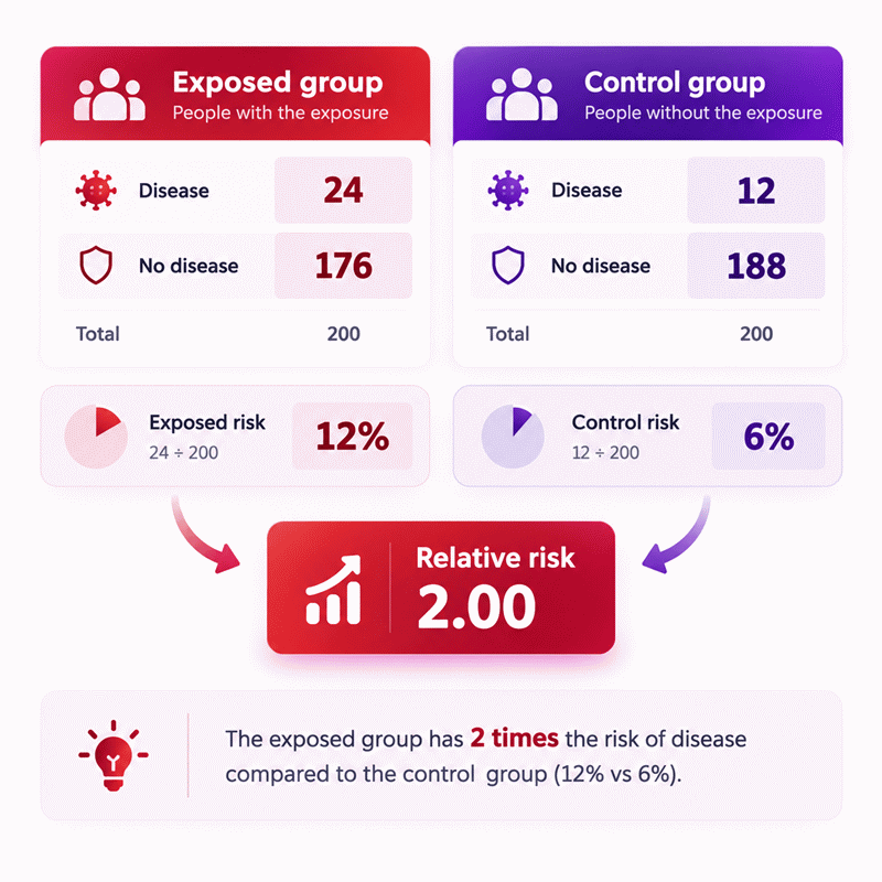
The exposed group has a disease risk of 12%, compared with 6% in the control group.
A relative risk of 2 means the observed exposed-group risk is twice the control risk.
The 95% confidence interval extends from approximately 1.0289 to 3.8876.
Because the complete interval is above 1, this dataset indicates an increased observed risk.
The calculator begins with one missing group count and a target relative risk of 2.
Rearranging the same relative-risk equation isolates b and produces a value of 176.
Substituting the solved count back into the original equation reproduces RR = 2 exactly.
The completed table can then be used normally to calculate the 95% confidence interval.
Results are rounded for display.
Internal calculations use full precision.
Calculations Disclaimer
What Does a Relative Risk Calculator Actually Tell You?
A researcher can have two clean groups and still misread the result. Relative risk solves one part of that problem. It compares the observed event probability between two groups. The first group is usually exposed, treated, or otherwise of interest. The second group provides the reference risk.
The number becomes useful only after the comparison direction is clear. A value near one means both observed risks are similar. A value above one means the numerator group has higher observed risk. A value below one means that group has lower observed risk. This simple structure makes the measure useful in many cohort studies and trials.
A Relative Risk Calculator removes repetitive arithmetic from that comparison. More importantly, it helps prevent simple transcription mistakes. Users can focus on what the data mean rather than moving numbers between several manual steps.
When Should You Use Relative Risk Instead of an Odds Ratio?
A common research problem starts before any number is calculated. The analyst must choose the right effect measure. Relative risk works naturally when event probability can be estimated in both comparison groups. This is often possible in prospective cohort studies and randomized trials.
An odds ratio answers a related but different question. It compares odds rather than probabilities. The distinction may appear small when events are rare. It can become important when events are common.
The safest choice begins with the study design. Ask whether each group’s event risk is directly observable from the data. If it is, a risk ratio can provide an intuitive comparison. If the sampling method fixes cases and controls, direct risks may not be available.
Why Study Design Changes the Correct Effect Measure
A student may see the same four-cell layout in two studies. That does not make both studies equivalent. The way participants entered the dataset matters. A cohort follows groups whose denominators carry real risk information. A traditional case-control design starts from outcome status instead.
This difference changes what the table can support. A calculation should therefore follow design logic, not visual appearance alone. A correct equation applied to the wrong design can still produce a misleading conclusion.
Good statistical work asks three questions first. How were participants selected? Can event probability be estimated? Which group is the intended reference? Those answers often determine the appropriate measure before any calculator is opened.
How Do You Read a 2×2 Risk Table Without Mixing Up the Groups?
A surprisingly common error is placing a correct number in the wrong cell. The arithmetic may then run perfectly while answering the wrong question. A 2×2 table should be read by both group and outcome.
One dimension separates the comparison groups. The other separates event from non-event observations. Every participant should belong to the correct combination. The total for each group must represent the population from which that group’s event risk is estimated.
The direction also matters. Exposed versus control is not interchangeable in interpretation. Swapping the groups changes which population becomes the reference. Before entering numbers, state the comparison in plain language. That one sentence can prevent a large interpretation error later.
What Counts as Exposed, Control, Event and No Event?
A clinical trial may use treatment and control instead of exposed and unexposed. An occupational study may compare workers with and without an exposure. A public-health investigation may compare people who encountered a suspected factor with those who did not.
The event should also be defined before analysis. It might be disease, recovery, relapse, injury, infection, or another binary outcome. The word “risk” does not require the event to be harmful. What matters is that the same event definition applies to both groups.
The control group is not automatically “healthy” or “untreated.” It is the comparison group defined by the research question. Clear labels make the final RR much easier to interpret.
How Should You Interpret RR Above, Below or Equal to 1?
A result can look dramatic simply because it is shown without context. Relative risk uses one as its natural reference point. That makes the direction easy to read but not always easy to judge.
An RR above one means the observed event risk is higher in the numerator group. An RR below one means it is lower. An RR equal to one means the observed risks are equal. These statements describe the comparison in the entered data.
They do not tell you whether the relationship is causal. They also do not tell you whether the absolute difference is large. Those questions require more information about baseline risk, design quality and uncertainty.
What Does a Relative Risk of 2 Mean?
A reader may see “2” and assume the event became two hundred percent more likely. That is a common wording error. A relative risk of two means the observed risk is twice the reference risk. This corresponds to a one-hundred-percent relative increase from the reference level.
The practical effect still depends on the starting risk. Doubling a very rare event may create a small absolute change. Doubling a common event can create a much larger absolute change. The ratio alone cannot show that distinction.
For clear communication, describe both direction and scale. Then check the underlying event risks before drawing practical conclusions.
What Does a Relative Risk of 0.5 Mean?
A value below one can be misread because readers often expect “risk” to increase. An RR of 0.5 means the numerator group’s observed risk is half the reference risk. It can also be described as a fifty-percent relative reduction.
That description still needs context. A fifty-percent relative reduction can represent a tiny or substantial absolute difference. The baseline level determines the practical size.
Words such as “protective” should also be used carefully. A lower observed risk is an association. Whether an exposure genuinely causes protection depends on the research design, bias control and broader evidence.
Why Does the Confidence Interval Matter?
Two studies can report the same point estimate and still provide very different evidence. The confidence interval helps show that difference. It describes the statistical precision surrounding the estimated effect under the method being used.
A narrow interval gives a more concentrated range of values compatible with the sampling model. A wide interval indicates greater imprecision. This is why reporting only the RR can hide important information.
The interval should be read beside the point estimate. It should not be treated as a guarantee about the population. It also cannot measure every source of uncertainty. Bias, poor measurement and confounding may remain even when the interval is narrow.
What Does It Mean When the Confidence Interval Includes 1?
A researcher may obtain an RR above one and expect a definitive positive association. The interval can complicate that conclusion. If the selected confidence interval includes one, the data remain statistically compatible with the null value under that interval procedure.
This does not prove that the groups are identical. It means the available data do not separate the estimated effect from the null value at that confidence level. The width of the interval also matters.
A broad interval can include both meaningful increases and meaningful decreases. That situation calls for cautious interpretation rather than a binary “effect” or “no effect” statement.
Why Do Larger Samples Often Produce Narrower Confidence Intervals?
A small study may produce an impressive RR but leave a wide range of uncertainty. More informative samples often reduce random sampling variability. The point estimate can stay similar while its interval becomes narrower.
This does not mean sample size fixes every problem. A large biased study can produce a precise estimate of the wrong quantity. Data quality, group definition and study design still matter.
Think of sample size as one part of precision. Event frequency matters too. Sparse outcomes can leave substantial uncertainty even when the overall number of participants appears large.
How Does Reverse Solving Work in a Relative Risk Calculator?
A practical problem sometimes starts with a target RR rather than a complete table. Perhaps three cell values are known and one count must be reconstructed. A bidirectional calculator can solve that missing value when the available information defines a unique solution.
This is an algebraic operation, not a new statistical model. The calculator uses the same relationship that connects the two group risks. It simply treats a different quantity as unknown.
This feature is useful for checking examples, validating datasets and exploring scenarios. It should not turn reconstructed values into observed evidence. A solved value remains derived from the assumptions and numbers provided by the user.
When Can a Missing 2×2 Cell Be Solved From Relative Risk?
A user may know three counts and the required risk ratio. In that setting, enough information can sometimes exist to determine the fourth count. The solution must still satisfy the logical structure of the table.
A valid result cannot create an impossible group size or an invalid event relationship. In real count data, researchers should also ask whether the reconstructed number makes sense as an observation count.
Reverse solving is strongest as a verification tool. It helps answer, “Which missing value would make these quantities consistent?” It does not answer, “What actually happened in the original study?” unless that value is independently confirmed.
Why Can Some Reverse Problems Have No Unique Answer?
An inverse problem can look solvable while lacking enough independent information. Several different datasets may sometimes create the same summary quantity. In other cases, the requested combination may have no valid solution.
A trustworthy calculator should not silently choose one answer. It should identify ambiguity or reject impossible combinations. This behavior is especially important when users edit derived statistical limits instead of a direct risk ratio.
Reverse calculation therefore needs stricter validation than ordinary forward calculation. A blank result with a useful explanation is safer than a plausible-looking value created from insufficient information.
Relative Risk vs Absolute Risk: What Can Decision Makers Miss?
A headline can say that risk doubled while hiding a very small baseline probability. Relative risk measures proportional change. It does not show the absolute number of additional events by itself.
This matters in medicine, public health, safety and policy. A large relative change from a tiny baseline can remain small in absolute terms. A modest relative change from a high baseline can affect many people.
Decision makers should therefore avoid reading RR in isolation. Check the risks in both groups. Ask how important the event is. Then consider statistical uncertainty and study quality. Relative and absolute perspectives answer different questions, and both can matter.
How Is Relative Risk Used in Cohort Studies and Randomized Trials?
A cohort study often begins with groups defined by exposure. Researchers then observe whether the outcome occurs. Because the group denominators are meaningful, event risks can be estimated directly and compared.
A randomized trial can provide a similar structure. Participants are allocated to intervention groups, and binary outcomes are observed. Risk ratios can then express proportional differences between groups.
The labels should match the actual question. “Exposed” may mean treatment, behavior, environmental factor or another condition. “Control” may represent placebo, usual care, no exposure or another valid comparison. Clear labeling prevents the statistical result from being separated from its research meaning.
When Is Relative Risk the Wrong Measure?
A calculator becomes dangerous when users assume every four-number dataset supports the same statistic. Relative risk requires group risks that have a defensible meaning. Some designs do not provide that information directly.
Case-control studies are an important example. Person-time data are another. Time-to-event data with censoring may require methods designed for survival analysis. Cross-sectional analyses may focus on prevalence rather than incidence.
The correct question is not “Can I force these values into a calculator?” It is “Does this statistic match how my data were generated?” That decision should come before interpretation.
Why Are Odds Ratios Common in Case-Control Studies?
A case-control study usually selects participants based on whether the outcome occurred. That sampling process means the observed case proportion does not represent population risk in the usual way.
Odds ratios remain estimable from the exposure distribution in cases and controls. For that reason, they are commonly associated with case-control designs. The odds ratio may resemble relative risk when outcomes are rare, but the two quantities are not generally identical.
Reporting should use the correct terminology. Calling an odds ratio a relative risk can exaggerate or distort the apparent effect when the outcome is common.
Why Does Person-Time Require a Different Risk Measure?
Some studies follow participants for very different lengths of time. A simple proportion may then ignore important exposure time. Person-time methods account for how long participants were observed and at risk.
These analyses typically use incidence rates and rate ratios rather than the simple risk ratio calculated from cumulative event proportions. The distinction is especially important when follow-up differs substantially or when repeated event opportunities matter.
Before using a Relative Risk Calculator, check whether your denominators are people observed over a defined period or units of person-time. They represent different statistical structures.
Which Common Mistakes Can Distort Relative Risk?
The most damaging errors are often simple. Groups may be reversed. Event and non-event counts may be swapped. A case-control table may be treated like a cohort table. A relative percentage may be confused with an absolute percentage-point change.
Other errors are less visible. Confounding can create an association that does not represent a causal effect. Selection can make groups unrepresentative. Misclassification can move observations into the wrong cells.
A calculator cannot detect every design problem. It can check numeric consistency, but it cannot know whether exposure was measured well. Statistical output should therefore remain connected to the study that generated it.
How Do Group Reversal, Sparse Events and Confounding Change Interpretation?
Reversing groups changes the comparison direction. The result may become the reciprocal of the original ratio. The underlying data stay the same, but the sentence used to describe them changes.
Sparse events create another challenge. Very small counts can make estimates unstable and intervals wide. Zero events can also create mathematical problems for common log-based methods.
Confounding is different. It is not solved by arithmetic. A third factor may be related to both exposure and outcome. Proper design or adjusted statistical models may be needed before a causal interpretation is reasonable.
How Should Relative Risk Be Reported Clearly in Research?
A useful report should allow another reader to understand both the result and its direction. State which group appears in the numerator. Identify the reference group. Define the outcome. Report the relative risk together with its confidence interval.
Include the underlying group risks when they improve practical interpretation. Avoid presenting a relative change as though it were an absolute change. Avoid causal wording unless the study design and evidence support it.
Clear reporting is not about making the number sound larger. It is about making the comparison reproducible. A reader should know what was compared, which outcome was counted, how uncertain the estimate is, and what the result cannot establish.
AxiCalculator is designed to make that first statistical check faster. Use the result as a transparent analytical step, then connect it back to the study design, source data and real decision being made.
Frequently Asked Questions
Can a relative risk ever be negative?
What happens if I swap the exposed and control groups?
Does a larger relative risk always mean a larger real-world effect?
Why can two datasets produce the same RR but different confidence intervals?
Can I use this RR method when observations are paired or clustered?
When should I avoid relying on a simple log-based RR confidence interval?
Is a count produced by reverse solving equivalent to an observed study count?
Our engineers are here to help you get it right.