Sensitivity and Specificity Calculator
- Last formula update:

Decimal & Rounding Policy
- Calculations use unrounded internal values to preserve statistical precision.
- Percentage results display up to two decimal places.
- Proportions and likelihood ratios display up to six decimal places.
- Reverse-solved counts display up to six decimals when fractional.
- Trailing zeros are omitted without changing the calculated value.
- Unit changes preserve the underlying value before reformatting.
- Excel formulas use full stored values instead of rounded display text.
Valid range
- TP, FP, FN, and TN accept values from 0 to 1,000,000,000,000.
- Prevalence accepts 0% to 100%, or a proportion from 0 to 1.
- Sensitivity and specificity accept 0% to 100%, or 0 to 1.
- PPV, NPV, and accuracy accept 0% to 100%, or 0 to 1.
- LR+ and LR- accept nonnegative values up to 1,000,000,000,000.
- A calculated LR+ may be infinite when specificity equals 100%.
- TP plus FN must exceed zero before sensitivity can be calculated.
- FP plus TN must exceed zero before specificity can be calculated.
- The total confusion-matrix count must exceed zero for accuracy.
- Every reverse-solved count must remain nonnegative and within range.

Wylena Brantford
Reviewers:
Valdren Clyforde
Zenara Dentwick
Check our editorial policy
September 26, 2026
1.0.0
Initial calculator and formula release.
Our engineers are here to help you get it right.
What Does a Sensitivity and Specificity Calculator Tell You?
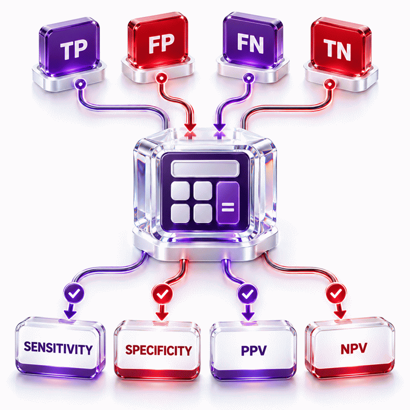
A Sensitivity and Specificity Calculator turns diagnostic counts into clear measures of test performance. It separates true positives, false positives, false negatives, and true negatives before calculating linked results. This matters because one accuracy percentage can hide serious errors.
- Sensitivity shows how often condition-positive cases are detected.
- Specificity shows how often condition-negative cases are cleared.
- PPV estimates how often a positive result is correct.
- NPV estimates how often a negative result is correct.
- Likelihood ratios describe the evidence strength of each result.
- Accuracy summarizes correct classifications within the entered sample.
Prevalence changes PPV and NPV, even when test characteristics stay fixed. A rare condition may produce more false positives than true positives. A Sensitivity and Specificity Calculator therefore needs the correct target-population prevalence.
AxiCalculator also supports reverse solving. Users can enter compatible results and recover a missing count or metric. Fractional reverse counts represent algebraic requirements, not partial observations. Review the sample, threshold, reference standard, and population before using any result in research or professional decisions. Use scenario testing to compare changing prevalence, inspect unexpected extremes, and catch inconsistent entries before results are copied into reports, presentations, or study plans safely.
Assumptions used in this calculator
- Test outcomes are classified against a valid reference standard.
- Counts represent mutually exclusive observations from the same evaluated sample.
- True and false classifications use the same positivity threshold.
- Sensitivity and specificity are proportions between zero and one.
- Prevalence describes the target population at the relevant evaluation time.
- Predictive values use entered prevalence, not the sample case fraction.
- Accuracy uses the entered confusion-matrix counts only.
- Count inputs are nonnegative and may include algebraic fractional results.
- Observed clinical counts should normally be whole numbers.
- Likelihood ratios are nonnegative and dimensionless.
- Undefined zero-denominator results are not replaced with correction factors.
- Calculations provide point estimates without confidence intervals or uncertainty modeling.
- Results support evaluation and do not replace clinical judgment.
Results are rounded for display.
Internal calculations use full precision.
Formulas Used in Sensitivity and Specificity Calculator :
Sensitivity
Specificity
Positive Likelihood Ratio
Negative Likelihood Ratio
Positive Predictive Value
Negative Predictive Value
Accuracy
- TP
- True positive count
- FP
- False positive count
- FN
- False negative count
- TN
- True negative count
- p
- Target-population prevalence as a proportion
- Se
- Sensitivity as a proportion
- Sp
- Specificity as a proportion
- LR+
- Positive likelihood ratio
- LR-
- Negative likelihood ratio
- PPV
- Positive predictive value
- NPV
- Negative predictive value
- A
- Accuracy as a proportion
Variables & Definitions
View a complete list of all variables used in this calculator, including definitions and units
Sensitivity and Specificity Calculator Variables and Statistical Measures
| Variable | Symbol | Base Unit | Valid Range | Definition |
|---|---|---|---|---|
| True positive | TP | Cases | 0 to 1,000,000,000,000 | Condition-positive observations correctly classified as positive. |
| False positive | FP | Cases | 0 to 1,000,000,000,000 | Condition-negative observations incorrectly classified as positive. |
| False negative | FN | Cases | 0 to 1,000,000,000,000 | Condition-positive observations incorrectly classified as negative. |
| True negative | TN | Cases | 0 to 1,000,000,000,000 | Condition-negative observations correctly classified as negative. |
| Prevalence | p | Proportion | 0 to 1 | Proportion of the target population with the condition. |
| Sensitivity | Se | Proportion | 0 to 1 | Probability of a positive result when the condition is present. |
| Specificity | Sp | Proportion | 0 to 1 | Probability of a negative result when the condition is absent. |
| Positive likelihood ratio | LR+ | Dimensionless ratio | 0 or greater | Change in diagnostic odds produced by a positive result. |
| Negative likelihood ratio | LR- | Dimensionless ratio | 0 or greater | Change in diagnostic odds produced by a negative result. |
| Positive predictive value | PPV | Proportion | 0 to 1 | Probability that a positive result represents the condition. |
| Negative predictive value | NPV | Proportion | 0 to 1 | Probability that a negative result represents no condition. |
| Accuracy | A | Proportion | 0 to 1 | Proportion of all observations classified correctly. |
Unit Conversion Table
Count Unit Conversion Table
| Unit Group | Unit Name | Symbol | Equivalent in Cases | Used For |
|---|---|---|---|---|
| Popular Units | Case | cases | 1 case | TP, FP, FN, and TN |
| Scientific Units | Observation | observations | 1 case | TP, FP, FN, and TN |
Probability Unit Conversion Table
| Unit Group | Unit Name | Symbol | Equivalent in Proportion | Used For |
|---|---|---|---|---|
| Popular Units | Percent | % | 1% = 0.01 | Prevalence, sensitivity, specificity, PPV, NPV, and accuracy |
| Scientific Units | Proportion | proportion | 1 proportion = 1 | Prevalence, sensitivity, specificity, PPV, NPV, and accuracy |
Likelihood Ratio Unit Conversion Table
| Unit Group | Unit Name | Symbol | Equivalent in Dimensionless Value | Used For |
|---|---|---|---|---|
| Popular Units | Ratio | ratio | 1 ratio = 1 | LR+ and LR- |
| Scientific Units | Dimensionless Value | 1 | 1 = 1 ratio | LR+ and LR- |
Example Calculation
The confusion matrix produces equal 90% sensitivity and specificity. The 8% prevalence lowers the positive predictive value despite strong test performance. The negative predictive value remains high in this modeled population. Accuracy reflects the entered sample counts and equals 90%.
Sensitivity and the true-positive count are known. The false-negative count is the only missing term. Rearranging the same sensitivity identity produces 16 false negatives. Fractional reverse results may occur when values do not represent whole observations.
Results are rounded for display.
Internal calculations use full precision.
Calculations Disclaimer
Why Can a Strong Diagnostic Test Still Mislead?
A screening team can report impressive accuracy and still create harmful confusion. The problem often begins with one attractive percentage. That figure may hide missed cases, false alarms, or population differences. A Sensitivity and Specificity Calculator separates those risks instead of blending them. The Sensitivity and Specificity Calculator also keeps each error type visible.
Sensitivity asks how often the test detects people with the condition. Specificity asks how often it clears people without the condition. Neither question starts with the observed test result. That distinction surprises many readers. It also explains why sensitivity cannot directly answer whether a positive result is correct.
A positive result needs a population-aware measure. A negative result needs one too. Positive predictive value and negative predictive value provide those views. Their meaning changes when prevalence changes. A result from one clinic may not transfer safely elsewhere.
AxiCalculator keeps these measures visible together. That layout reduces a common reasoning error. Users can see test performance, predictive meaning, and overall classification accuracy without switching tools. Editable results also support reverse analysis when one quantity is missing.
Pause here: high sensitivity does not guarantee a trustworthy positive result.
What Does the Calculator Reveal Beyond One Accuracy Score?
A laboratory report may show 95% accuracy and still hide an uneven failure pattern. Accuracy counts every correct classification together. It does not show which group carries the errors. This can matter when missed cases have greater consequences than false alarms.
The calculator separates seven connected measures. Sensitivity and specificity describe conditional performance. Likelihood ratios describe evidence strength. Predictive values describe result credibility at a stated prevalence. Accuracy summarizes the entered sample.
These outputs answer different questions. They should not compete for one universal winner. A screening program may prioritize sensitivity. A confirmatory workflow may demand stronger specificity. A patient-facing interpretation usually needs predictive values or post-test probability.
The raw counts remain essential. They expose sample size and error distribution. Two studies can show the same sensitivity with very different evidence strength. Ninety correct detections among one hundred cases differ from nine among ten cases.
How Sensitivity Exposes Missed Positive Cases
A missed case can delay action even when most test results look correct. Sensitivity focuses only on observations where the condition is present. It compares detected cases with all reference-positive cases.
High sensitivity means fewer false negatives within that group. It does not describe false positives. It also does not promise that every positive result is correct. Those questions require specificity and predictive value.
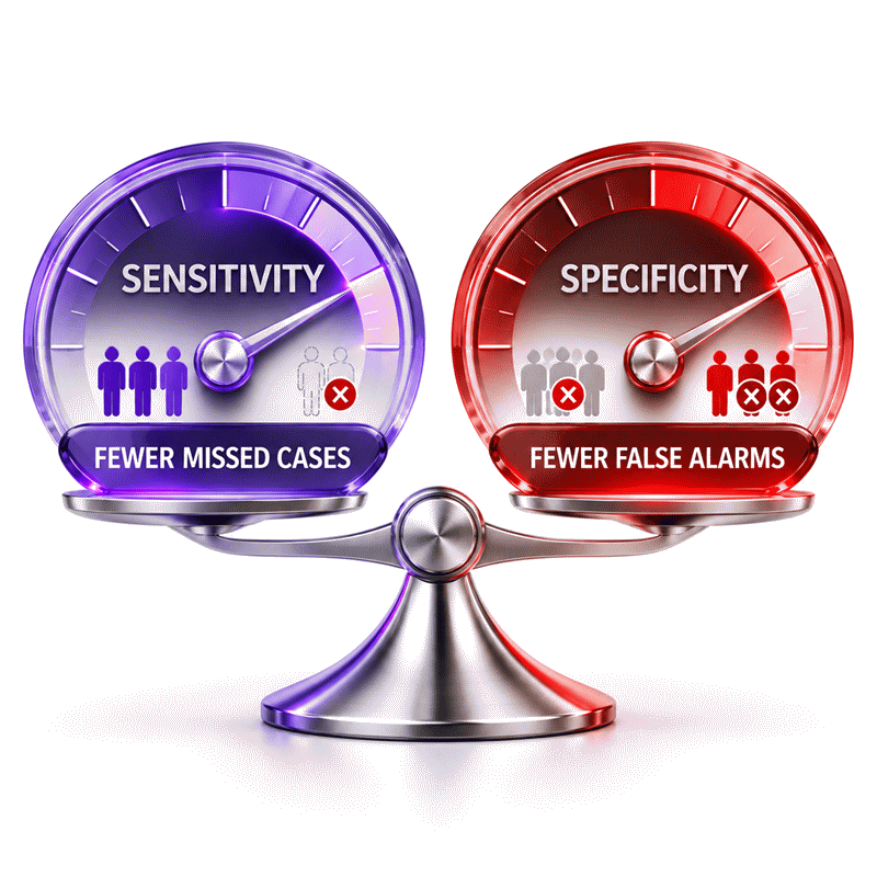
Thresholds can change sensitivity. A permissive threshold may capture more true cases. It may also classify more condition-negative observations as positive. The gain therefore has a cost.
When evaluating sensitivity, review the number of positive reference cases. A perfect value from a tiny sample can be unstable. The point estimate is mathematically correct for that table. The wider evidence may remain uncertain.
How Specificity Exposes False Positive Results
False alarms can trigger repeat testing, anxiety, cost, and unnecessary intervention. Specificity focuses on observations where the condition is absent. It measures how often the test correctly returns a negative classification.
High specificity means fewer false positives in that reference-negative group. It does not measure missed disease. It also cannot show positive-result credibility without prevalence.
A stricter threshold may improve specificity. However, it can also increase false negatives. That tradeoff should match the intended role of the test. Screening and confirmation often need different balances.
Always verify which table cell contains false positives. Transposed matrices are common. They can produce believable numbers with reversed meaning. Clear labels protect the entire calculation.
How Does the 2×2 Table Control Every Result?
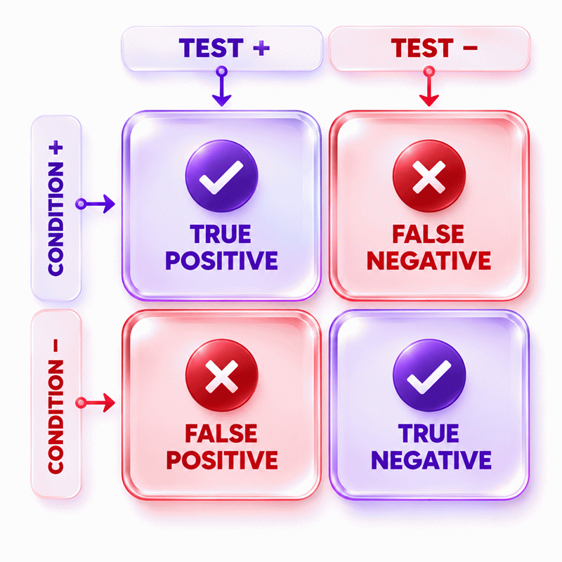
A copied spreadsheet can swap rows or columns without showing an obvious error. The four-cell table prevents that mistake when labels remain explicit. Each observation belongs to one test outcome and one reference condition.
Condition present + Test positive → True positive
Condition present + Test negative → False negative
Condition absent + Test positive → False positive
Condition absent + Test negative → True negative
True positives and false negatives form the condition-positive group. False positives and true negatives form the condition-negative group. Sensitivity and specificity use those separate denominators.
Predictive questions turn the table in another direction. Positive-result credibility compares true positives with all positive results. Negative-result credibility compares true negatives with all negative results. When external prevalence is supplied, Bayesian weighting recreates those population-level meanings.
All four counts should come from one compatible evaluation. Mixing thresholds, dates, laboratories, or patient groups breaks the table. The calculator cannot detect every design mismatch. Data preparation remains a human responsibility.
Why Does Prevalence Change the Meaning of a Result?
Two hospitals can use the same test and report different positive predictive values. Their patient populations may carry different baseline risk. Prevalence controls how many true cases exist before the test acts.
When a condition is rare, the pool without the condition becomes large. Even a small false-positive rate can create many false alarms. Positive predictive value can therefore remain modest despite strong sensitivity and specificity.
When prevalence rises, positive results usually become more credible. Negative results usually become less reassuring. The test characteristics may stay unchanged. The population meaning still moves.
Lower prevalence → fewer true cases → lower PPV → higher NPV
Higher prevalence → more true cases → higher PPV → lower NPV
The correct prevalence should match the intended population and time. A national estimate may not suit a referral clinic. An old estimate may not fit a changing outbreak. Document the source and relevance before interpreting predictive values.
Conditional probability updates a starting risk with new test evidence. Predictive values apply that logic to positive and negative results.
Why Rare Conditions Create More False-Alarm Pressure
A rare condition creates a large condition-negative population. That population gives false positives more opportunities to appear. The absolute count can exceed true positives even with good specificity.
This is the core false-positive paradox. It does not mean the test is useless. It means the positive result needs context and often confirmation. The cost of confirmation should be planned before broad screening begins.
Users should test several plausible prevalence values. Scenario analysis reveals how stable the interpretation remains. A result that changes sharply deserves cautious communication.
What Do Likelihood Ratios Add?
A result may need to update an existing probability rather than describe a whole population. Likelihood ratios provide that bridge. They combine sensitivity and specificity into result-specific evidence strength.
LR+ describes positive evidence. Larger values produce stronger upward shifts in odds. LR- describes negative evidence. Smaller values produce stronger downward shifts.
A ratio near one provides little change. This simple boundary helps readers avoid overreacting. A statistically measured result may still add almost no diagnostic information.
Likelihood ratios are often more portable than predictive values. They do not directly contain prevalence. However, portability is not automatic. Threshold, spectrum, procedure, and reference quality can still change them.
When Positive Evidence Becomes Persuasive
A positive result can look decisive because the interface uses a clear label. The evidence may still be weak. LR+ checks how much more often that result occurs with the condition.
Moderate evidence can matter when prior probability is already meaningful. The same ratio may remain insufficient from a tiny starting probability. Always connect evidence strength with the starting context.
When Negative Evidence Becomes Reassuring
A negative result can feel final while residual risk remains important. LR- shows how strongly that result lowers odds. Values near zero provide stronger negative evidence.
A weak LR- may leave meaningful risk after testing. Further evaluation may still be justified. The calculator supports statistical understanding, while decisions require qualified context.
Why Can Accuracy Hide a Weak Classifier?
An imbalanced dataset can reward the most common prediction. Imagine a rare condition within a huge screening population. A model can label everyone negative and appear highly accurate.
That model has poor case detection. Accuracy alone hides the failure because true negatives dominate the total. Sensitivity immediately exposes the missed cases.
Machine-learning teams face the same issue. Precision, recall, specificity, and class prevalence should travel with accuracy. The classification threshold must also be reported.
High accuracy can describe class imbalance rather than useful discrimination.
How Does Reverse Solving Support Planning?
A study designer may know a target sensitivity but lack one count. A forward-only calculator cannot answer that planning question. Reverse solving rearranges the same statistical identities.
AxiCalculator lets an editable result become a known value. When enough compatible values exist, the missing count or metric is recovered. This supports teaching, audits, scenario checks, and early design work.
The answer may be fractional. That does not represent part of a patient. It describes an algebraic requirement. Researchers should test nearby whole counts and recalculate the achieved performance.
Some combinations cannot identify one unique answer. Others create impossible negative counts. Clear error states are better than a forced number. They tell the user that more information is required.
Why Input Order Should Not Change the Answer
An interactive solver can become confusing when field order changes its behavior. A constraint-based approach evaluates all compatible relationships together. The mathematical answer should depend on values, not typing order.
Entered values remain fixed unless the user changes them. Derived values stay visibly marked. A conflict warning appears when the fixed set cannot satisfy one model.
Which Study Choices Change Observed Performance?
A calculator can reproduce a table perfectly while the study remains biased. The index test must be compared with a defensible reference standard. Otherwise, classifications may represent agreement rather than truth.
Spectrum effects also matter. Performance in severe cases and healthy controls may exceed performance near clinical decision boundaries. Real populations often contain harder cases.
Verification bias appears when reference testing depends on the index result. Positive and negative groups then receive different confirmation. The final table can become distorted.
Timing matters too. A condition can change between tests. Sample handling can also change results. The four counts cannot explain these procedural errors.
Correct implementation differs from real-world suitability. Diagnostic studies must separate accurate calculation from valid evidence.
Why Small Samples Produce Fragile Extremes
A small study can report perfect sensitivity because no miss occurred. One additional false negative may change the estimate sharply. The same risk applies to specificity.
Point estimates need sample context. Counts make that context visible. Formal reports should add suitable uncertainty intervals and study-design details.
How Should Results Be Communicated?
A polished percentage can travel farther than its assumptions. Good reporting keeps the evidence attached. Start with the four counts and tested population.
State the threshold and reference standard. Report the study setting and sampling method. Identify whether prevalence came from the sample or an external population.
Separate observed metrics from modeled predictive values. Avoid calling any result universal. Describe what the number answers and what it does not answer.
Counts show what happened.
Rates show conditional performance.
Prevalence shows population context.
Likelihood ratios show evidence strength.
How to Avoid the Most Common Interpretation Errors
A common error treats sensitivity as positive-result credibility. Another treats specificity as negative-result credibility. These pairs condition on different groups.
Another error transports PPV without prevalence. A third reports accuracy without class balance. A fourth rounds intermediate values before completing linked calculations.
Use the visible metric names as questions. Ask which group forms each denominator. That habit catches many errors before publication.
How Can AxiCalculator Support a Transparent Workflow?
A busy researcher may need an answer, an audit trail, and a shareable state. AxiCalculator combines those tasks within one local workflow. Results update while compatible values are entered.
Editable outputs support reverse solving. Independent unit controls preserve the underlying value. Share links store only the required calculator state.
PDF export creates a readable record. Excel export provides a forward formula model for review. These features improve communication without turning the result into clinical advice.
Use the calculator to check relationships and expose inconsistencies. Then verify important decisions against study protocols and qualified expertise. Transparent calculation is a strong start, not the final validation step.
Open AxiCalculator, enter the evidence you trust, and inspect every linked result.
Frequently Asked Questions
Why can two populations get different predictive values from the same test?
What should I check before entering a confusion matrix?
Why is overall accuracy sometimes a poor summary?
Can this calculator be used for machine-learning classification?
How should zero cells be handled in a diagnostic study?
Why can reverse solving produce a fractional diagnostic count?
What must be reported when prevalence is supplied externally?
Our engineers are here to help you get it right.