Bayes’ Theorem Calculator
- Last formula update:

Decimal & Rounding Policy
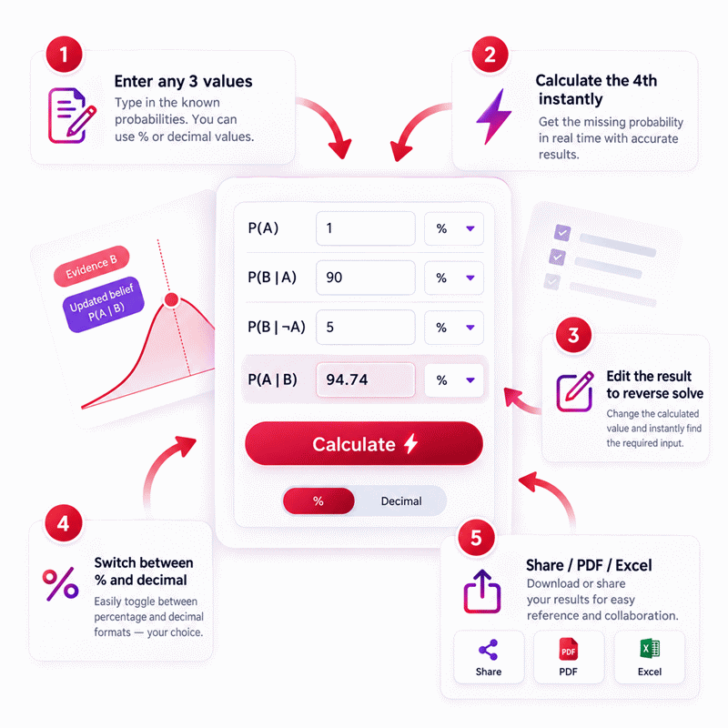
- Probability inputs may be entered as percentages or decimal values.
- Percentage values are converted to decimal probabilities before calculation.
- Intermediate probability calculations are not rounded.
- Displayed results use up to 12 significant digits when needed.
- Rounding is applied only when formatting the displayed result.
Valid range
- P(A): Enter a probability from 0 to 1, or 0% to 100%.
- P(B): Enter a probability from 0 to 1, or 0% to 100%.
- P(B|A): Enter a conditional probability from 0 to 1, or 0% to 100%.
- P(A|B): Enter a conditional probability from 0 to 1, or 0% to 100%.
- P(B) must be greater than zero when calculating P(A|B).
- P(A) must be greater than zero when calculating P(B|A).
- P(B|A) must be greater than zero when reverse-solving P(A).
- P(A|B) must be greater than zero when reverse-solving P(B).
- Any calculated probability outside 0 to 1 indicates inconsistent input values.

Wylena Brantford
Reviewers:
Valdren Clyforde
Zenara Dentwick
Check our editorial policy
September 22, 2026
1.0.0
Initial calculator and formula release.
Our engineers are here to help you get it right.
How does a Bayes’ Theorem Calculator turn evidence into an updated probability?
Bayes’ Theorem Calculator results help you update a starting probability after new evidence appears. The tool is especially useful when three related probabilities are known and you need the fourth, including a reverse-solved value.
- Read every conditional probability in the correct direction.
- Use a starting probability from the relevant population.
- Do not treat a strong signal as proof.
- Use reverse solving to challenge missing or inconsistent inputs.
- Interpret posterior probability as uncertainty, not certainty.
- Check whether a rare base rate explains a surprising result.
- Compare plausible scenarios when source data is uncertain.
A Bayes’ Theorem Calculator can support statistics study, quality control, reliability analysis, fraud screening, classification, and evidence-based decisions. AxiCalculator reduces the arithmetic workload so you can focus on the probability model itself. The most useful result is not merely a number. It is a clearer view of how much the evidence should change your current belief and whether the data supporting that update belongs to the same real-world context.
Assumptions used in this calculator
- All entered values represent probabilities within one consistent event model.
- Probability inputs must remain between zero and one inclusive.
- Percentage values are converted to decimal probabilities before calculation.
- Conditional probabilities use the event order shown in their notation.
- Known probabilities are assumed internally consistent with Bayes’ theorem.
- The conditioning event must have positive probability when used as denominator.
- Reverse solving uses the same Bayes relationship as forward solving.
- Intermediate calculations retain floating-point precision without manual rounding.
- Display rounding does not change the mathematical relationship being evaluated.
- Inputs are treated as exact values unless uncertainty is separately assessed.
- Statistical sampling error is not estimated by this calculator.
- Event dependence is determined only by the probabilities users provide.
- Results are mathematical estimates, not guarantees of real-world outcomes.
Results are rounded for display.
Internal calculations use full precision.
Formulas Used in Bayes' Theorem Calculator :
Probability Normalization
Here, r is the numeric percentage value and p is its normalized decimal probability.
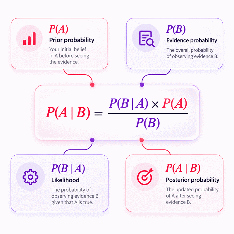
Bayes' Theorem Relationship
- P(A)
- Probability of event A.
- P(B)
- Probability of event B.
- P(B|A)
- Probability of event B given event A.
- P(A|B)
- Probability of event A given event B.
When one probability is unknown, the calculator algebraically isolates that term from this same relationship.
- Direct calculation of P(A|B) requires P(B) greater than zero.
- Reverse calculation of P(B|A) requires P(A) greater than zero.
- Reverse calculation of P(A) requires P(B|A) greater than zero.
- Reverse calculation of P(B) requires P(A|B) greater than zero.
Variables & Definitions
View a complete list of all variables used in this calculator, including definitions and units
Bayes' Theorem Calculator Variables and Probability Definitions
| Variable | Meaning | Valid Range | Calculator Role | Special Condition |
|---|---|---|---|---|
| P(A) | Probability that event A occurs. | 0 to 1, or 0% to 100% | Known value or reverse-calculated probability. | Must exceed zero when used to calculate P(B|A). |
| P(B) | Probability that event B occurs. | 0 to 1, or 0% to 100% | Known value or reverse-calculated probability. | Must exceed zero when used to calculate P(A|B). |
| P(B|A) | Probability of event B given that event A occurred. | 0 to 1, or 0% to 100% | Likelihood term or reverse-calculated probability. | Must exceed zero when reverse-solving P(A). |
| P(A|B) | Probability of event A given that event B occurred. | 0 to 1, or 0% to 100% | Posterior probability or reverse-calculated probability. | Must exceed zero when reverse-solving P(B). |
| p | Normalized decimal representation of a probability. | 0 to 1 | Internal calculation representation. | Obtained from percentage input before calculation. |
| r | Numeric percentage representation of a probability. | 0 to 100 | Percentage input and display representation. | Converted to decimal form before calculation. |
Unit Conversion Table
Percent Probability Conversion Table
| Unit Group | Unit Name | Symbol | Equivalent in Decimal Probability | Used For |
|---|---|---|---|---|
| Popular Units | Percent | % | 1% = 0.01 | Common probability input and result display. |
Decimal Probability Conversion Table
| Unit Group | Unit Name | Symbol | Equivalent in Percent | Used For |
|---|---|---|---|---|
| Scientific Units | Decimal Probability | 1 | 1 = 100% | Normalized probability calculations and scientific input. |
Example Calculation
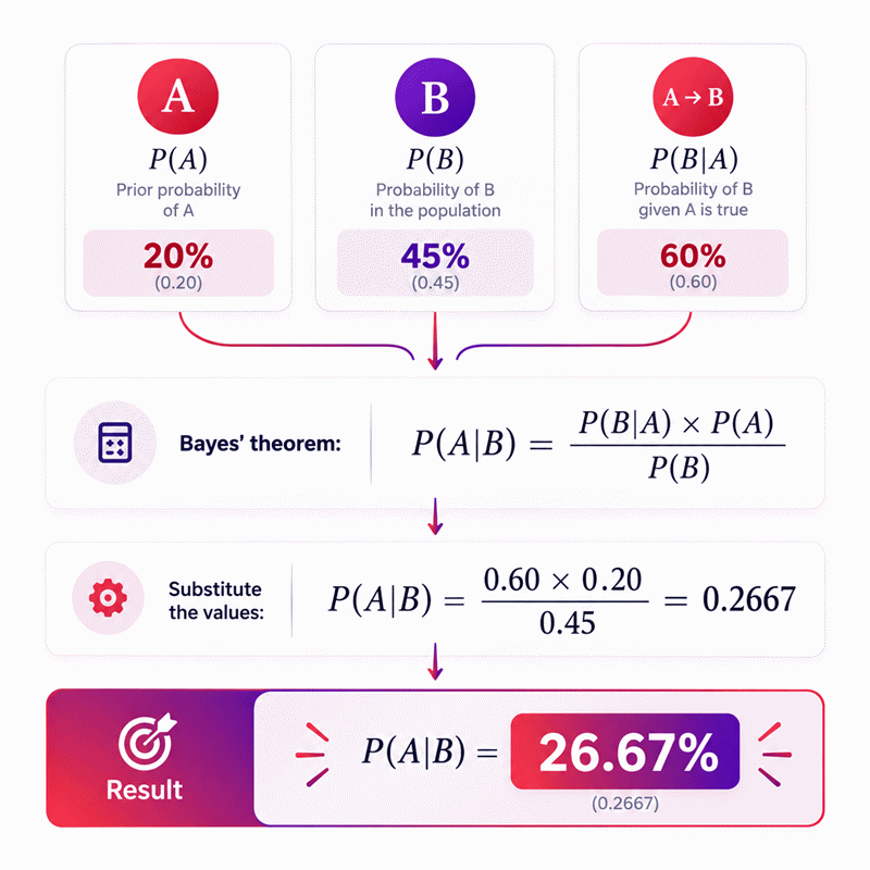
Assume event A represents a component defect and event B represents a sensor alarm.
The component defect rate is 18%, while alarms occur in 42% of observations.
A sensor alarm appears in 70% of observations where the defect is present.
After observing an alarm, the calculated probability of the defect becomes 30%.
Assume event A is unknown while the remaining three probabilities are available.
The observed event B occurs in 36% of cases.
The known conditional probabilities are 64% for P(B|A) and 40% for P(A|B).
Reverse solving the same Bayes relationship produces a prior probability of 22.5%.
Results are rounded for display.
Internal calculations use full precision.
Calculations Disclaimer
Why Can a Strong Signal Still Lead to a Low Probability?
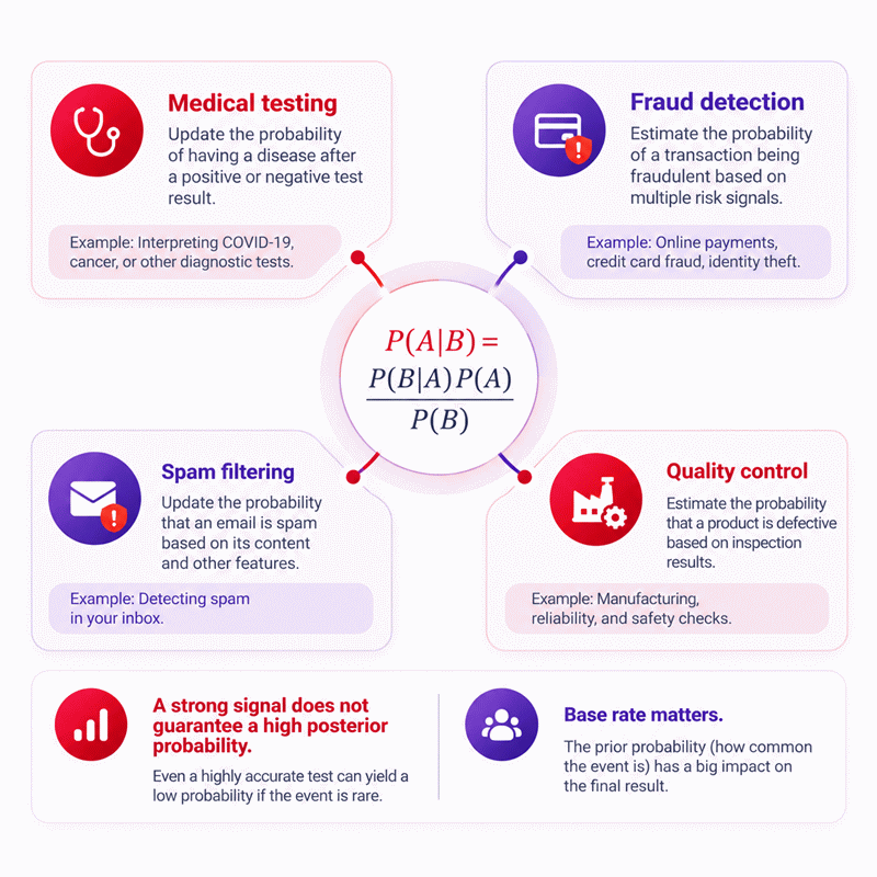
A real problem appears when a signal feels more convincing than it really is. A positive alert, a flagged transaction, or a failed quality check can look decisive. Yet the event behind that signal may still be uncommon. A Bayes’ Theorem Calculator separates emotional certainty from numerical evidence. It begins with what was plausible before the signal appeared. It then measures how well the signal fits the event. The probability is updated instead of treating the signal as proof.
This matters whenever false alarms are possible. A strong detector can still create many false positives when the target event is rare. A fraud alert can be technically sensitive while most alerts remain legitimate transactions. A manufacturing alarm can detect many defects while still reacting to acceptable parts. A screening signal can appear impressive until the underlying event frequency is considered.
The practical lesson is simple. Evidence only has meaning inside its probability context. Ignoring that context creates confident errors. A useful Bayesian workflow forces the starting probability and the evidence into the same decision. That single discipline makes the result easier to interpret and much harder to misuse.
The Base Rate Problem Behind Surprising Results
A real decision fails when the starting frequency is ignored. Teams often focus on how accurate a detector looks in isolation. They forget to ask how often the target event occurs at all. That starting frequency is the base rate. A rare event begins with a low prior probability. New evidence can raise it sharply without making it likely in absolute terms.
This is why rare defects, rare fraud patterns, rare failures, and uncommon classifications require careful interpretation. The result may feel unexpectedly low because human intuition tends to overweight vivid evidence. A Bayes’ Theorem Calculator keeps the starting probability visible instead of allowing the alert to dominate the decision.
The base rate also controls workload. A low-prevalence event can create many more false investigations than true discoveries. That cost matters in quality control, cybersecurity, finance, and screening systems. The better question is not only whether a detector catches the event. Ask how the event frequency changes what each alert actually means.
Why Inverse Probabilities Mislead Smart People
A common error begins with two sentences that sound almost identical. “The signal is likely when the event is present” is not the same as “the event is likely when the signal appears.” The condition changed. That change creates a different probability question.
Engineers, analysts, students, and managers all make this mistake. Ordinary language hides the direction of conditioning. A system may detect 95% of true defects, yet a detected item does not automatically have a 95% probability of being defective. The background frequency and competing sources of the signal still matter.
A useful workflow labels the event and evidence before entering any number. Write the meaning in plain language first. Then map each value to its probability notation. This prevents a mathematically correct calculation from answering the wrong real-world question.
How Does Evidence Change What You Should Believe?
A real investigation starts with uncertainty, not a blank slate. Some information already exists before new evidence arrives. It may come from historical production rates, previous tests, past transactions, earlier inspections, or a validated model. That information creates the starting probability.
New evidence should change that position only as much as it deserves. Evidence strongly associated with the event should move the probability more. Weak evidence should move it less. Evidence that fits alternative explanations can reduce the probability. This process prevents the latest observation from automatically becoming the most important observation.
The benefit is consistency. Two analysts using the same probability model should not reach opposite conclusions merely because one finds the evidence more dramatic. Bayesian updating provides a repeatable way to combine what was already known with what just happened.
From Starting Probability to Updated Probability
A practical workflow often needs one probability before evidence and another afterward. The first describes the event before the observation. The second reflects the updated view once the observation is known. The difference between them tells you how informative the evidence was under the model.
A large change deserves attention. It shows that the evidence strongly separates the target event from other explanations. A small change also contains useful information. It can show that the signal adds little beyond what was already known.
This is more useful than asking whether a signal is simply “good” or “bad.” A detector should be judged by how much meaningful information it adds to the decision. AxiCalculator makes that change easier to inspect without forcing users to perform the algebra manually.
When Evidence Adds Little Information
A weak signal creates a practical risk. People may act because something happened, even when that event barely changes the odds. If the evidence is almost equally common whether the target event is true or false, it provides little discrimination.
This can happen with noisy alarms, generic warning indicators, weak classification features, or broad screening rules. The updated probability then stays near its starting level. The correct response is not to force certainty. The correct response is to recognize that the evidence is not informative enough for a strong conclusion.
When Evidence Changes the Decision
A useful signal earns attention when it meaningfully separates one explanation from another. The updated probability may then cross an operational threshold. That threshold could trigger inspection, manual review, additional testing, escalation, or a different workflow.
Bayesian reasoning does not choose the threshold for you. The acceptable threshold depends on cost, safety, time, reversibility, and the consequences of errors. The calculator helps answer whether the evidence moved probability enough to justify considering the next step.
What Does P(A|B) Actually Mean in Plain English?
A real misunderstanding appears when notation is read too quickly. P(A|B) means the probability of A after B is known to have occurred. The vertical bar can be read as “given.” That small reading habit prevents large errors.
Suppose A represents a component defect. Let B represent a sensor alarm. P(A|B) asks how likely the component is defective after the alarm occurs. It does not ask how often the alarm appears when the component is defective. Those are different questions.
Clear naming matters because the symbols themselves carry no industrial meaning. Event A can represent a defect, fraudulent transaction, failure, spam message, or any other event. The notation only becomes useful when the event definitions are precise.
Reading the Condition in the Correct Direction
A real calculation can be numerically perfect yet conceptually wrong when the condition is reversed. Always read the expression from left to right: probability of the left event, given the event on the right.
This habit is especially important in diagnostics, anomaly detection, fraud alerts, and classification systems. A high detection rate does not automatically mean a high probability that every detected case is truly positive. The direction determines which group is being described.
Before calculating, translate each probability into one plain sentence. If the sentence does not match the data source, stop. Fixing the event definition is usually easier than explaining a misleading result later.
Separating Likelihood from Posterior Probability
A practical model becomes clearer when likelihood and posterior probability are not treated as synonyms. Likelihood describes how compatible the observed evidence is with an event or hypothesis. Posterior probability describes how plausible that event becomes after the evidence is observed.
The posterior depends on more than likelihood. The starting probability and the overall evidence context also matter. This explains why an impressive detector can produce a moderate final probability when the target event is rare.
This distinction also improves communication. Teams should not present a detector’s sensitivity as though it were the chance that an alert is correct. Those quantities answer different questions and can differ dramatically.
How Can Reverse Solving Expose a Bad Assumption?
A real audit often starts with a claimed result and asks what input would be required to produce it. Reverse solving makes that possible. Instead of always treating the posterior as unknown, another probability can become the missing value.
This is useful for sensitivity analysis, model review, homework verification, target setting, and technical QA. If the required missing probability becomes impossible, the target and known values cannot all belong to one consistent probability model.
That is valuable information. An impossible result is not merely an arithmetic inconvenience. It points toward incompatible assumptions, mismatched populations, incorrect transcription, or a misunderstanding of which conditional probability was supplied.
Finding a Missing Prior from Known Conditional Probabilities
A planning problem may ask what starting frequency would support a desired updated probability. Reverse solving can isolate that missing prior while the other probabilities remain fixed.
This is useful when reviewing ambitious claims. If the required starting rate differs greatly from observed history, the claimed posterior deserves further investigation. The result can expose where expectations and measured data have separated.
The same approach works in quality control, reliability planning, fraud monitoring, and statistical coursework. It turns the calculator into a consistency checker rather than a one-direction answer box.
Finding the Evidence Probability from the Same Relationship
A real report may provide a starting probability, a conditional signal rate, and a final probability while omitting how often the signal appears overall. Reverse solving can recover that missing evidence probability.
The recovered value can then be compared with operational data. A large mismatch may indicate a population shift, reporting error, or incompatible dataset. This check is particularly useful when probabilities were collected from separate dashboards or studies.
A result that is mathematically consistent but operationally implausible should not be ignored. It is a reason to inspect the data lineage before using the model for decisions.
Where Does Bayes’ Theorem Matter Outside the Classroom?
A real organization rarely labels its problem “Bayes theorem.” It sees alerts, inspections, defects, suspicious transactions, messages, warnings, tests, and uncertain causes. The same probability logic appears beneath all of them.
Bayesian reasoning becomes useful whenever a team starts with some probability and receives new evidence. That applies to manufacturing, reliability, cybersecurity, finance, analytics, machine learning, research, and many decision systems.
The symbols are less important than the workflow. Define the event. Define the evidence. Use data from compatible populations. Update the probability. Interpret the result in the context of a real action.
Quality Control and Defect Investigation
A factory problem often begins with an inspection signal rather than a confirmed defect. The signal may be sensitive but imperfect. Historical defect frequency supplies the starting context. Inspection behavior shows how often that signal appears when defects are present.
The updated probability can help prioritize manual checks or containment actions. However, the data should come from the same product family, production environment, and meaningful time period. Mixing rates from unrelated lines can produce a clean number with poor real-world meaning.
Bayesian thinking is therefore as much about data discipline as arithmetic. A calculator speeds the arithmetic. The engineering team still owns the process definition and the data quality.
Fraud Alerts, Spam Filters, and Classification
A classification problem often produces more alerts than true events. Fraud systems and spam filters face this constantly. A model can detect many true cases while also creating a large false-positive workload.
The base rate explains much of this behavior. When the target class is rare, even a small false-positive rate can generate many incorrect alerts. The posterior probability helps translate model behavior into a more meaningful case-level interpretation.
Teams should also watch population changes. Customer behavior, attack patterns, message content, and transaction mixes evolve. A probability model built on old distributions may remain mathematically correct while becoming less useful operationally.
Reliability Decisions Under Uncertainty
A reliability problem may involve a warning signal from a component, sensor, inspection process, or monitoring system. The warning is not the failure itself. It is evidence about a possible failure state.
Bayesian updating helps rank what deserves inspection next. It can improve troubleshooting order and maintenance prioritization. It does not replace physical diagnostics, engineering limits, or safety requirements.
The result is strongest when the probability model reflects the actual equipment population and recent operating conditions. Old fleet statistics may be misleading after a redesign, maintenance campaign, or environmental change.
Why Do Real Data Problems Break Simple Probability Intuition?
A real dataset rarely stays clean forever. Populations shift. Sensors age. User behavior changes. Suppliers change. Sampling rules evolve. A probability that represented last year’s system may no longer describe today’s system.
Bayes’ theorem remains mathematically valid. The danger lies in stale or incompatible inputs. This distinction separates a correct equation from a useful model.
A strong workflow therefore asks where each probability came from, when it was measured, and whether it applies to the current population. The calculator can update numbers instantly. It cannot automatically discover every hidden shift in the data-generating process.
Dependence, Selection Bias, and Shifting Populations
A real model can fail when evidence comes from a biased subset. Suppose alerts are investigated only for high-risk users. Conditional rates estimated from those investigations may not apply to ordinary users.
Dependence creates another risk. Two signals can appear to be separate pieces of evidence while sharing the same underlying cause. Treating them as independent can exaggerate confidence.
Population shift adds a third problem. A rate measured in one region, season, product revision, or customer segment may not transfer cleanly elsewhere. Good Bayesian analysis starts by checking data compatibility.
The Cost of Using the Wrong Base Rate
A wrong base rate creates a quiet error that can dominate the final interpretation. If the starting probability is too high, the result may look more alarming than reality. If it is too low, meaningful evidence may be discounted.
The cost can appear as unnecessary inspections, missed failures, wasted analyst time, poor triage, or inefficient resource allocation. The most relevant population should therefore define the starting rate.
When several base rates are plausible, compare the resulting outcomes. A sensitivity range often tells you more than pretending one uncertain input is exact.
How Should You Interpret a Bayes Result Before Acting?
A real decision needs more than a probability display. Ask what action the result is supposed to support. A 30% probability may justify a low-cost inspection. The same probability may be far too weak for an irreversible action.
Context changes the threshold. Cost, risk, reversibility, time pressure, and available alternatives all matter. Bayes helps quantify uncertainty. It does not choose your business, engineering, or ethical priorities.
A useful interpretation connects the updated probability to a defined next step. That prevents the calculator from becoming a decorative number generator.
Probability Is Not Certainty or Causation
A communication problem appears when probability is presented as proof. An 80% posterior still contains uncertainty. It also does not prove that the evidence caused the event.
Conditional probability describes relationships inside a probability model. Causal conclusions require additional evidence and a suitable causal design.
Precise language protects decisions. Say that an event became more or less likely. Avoid turning probabilistic results into statements of certainty unless certainty is actually justified.
Sensitivity Checks for Better Decisions
A real decision becomes more robust when more than one plausible input set is tested. Change the starting probability within a defensible range. Recalculate using alternative evidence rates when the data is uncertain.
Then watch whether the decision changes. If small input changes create large swings, the model is sensitive. That deserves caution. If the conclusion stays stable across realistic values, confidence improves.
This practice is often more valuable than displaying additional decimal places. Decision stability matters more than cosmetic precision.
What Makes a Bayes’ Theorem Calculator Worth Trusting?
A real calculator earns trust when its behavior is predictable, transparent, and easy to challenge. Users should know which probability is being solved and what each value means.
The tool should reject impossible states instead of confidently displaying nonsense. Reverse solving should use the same probability relationship rather than a hidden alternative method. Results should update consistently when known values change.
AxiCalculator is most useful when it removes arithmetic friction without hiding uncertainty. The tool should help users inspect assumptions, compare probability states, and identify inconsistent data. Trust comes from clear behavior, honest limits, and results that users can independently challenge.
Frequently Asked Questions
Why can the same test result mean different things for two populations?
Can I compare two Bayes results created from different data sources?
What should I do when a Bayesian result feels completely counterintuitive?
Can a posterior probability be used as a decision threshold by itself?
How should an engineer use Bayesian updating when sensor alarms are correlated?
How can reverse solving validate a quality-control probability claim?
What is the safest way to use Bayesian probabilities in a changing production process?
Our engineers are here to help you get it right.