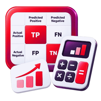
Confusion Matrix Variables
- Last formula update:
Decimal & Rounding Policy
- Calculations use full available precision and never round intermediate values.
- Displayed results use up to six decimal places with unnecessary trailing zeros removed.
- Percentage results are converted from the full-precision ratio before display rounding.
- Reverse calculations use unrounded values to reduce accumulated numerical error.
- Matthews correlation coefficient calculations retain full precision before final formatting.
- Undefined ratios remain undefined instead of being rounded or replaced with zero.
- Values extremely close to negative zero are displayed as zero.
Valid range
- TP, FP, FN, and TN accept finite nonnegative values from 0 to 9,007,199,254,740,991.
- Ordinary observation counts are typically integers, while fractional values may represent weighted observations.
- Accuracy, precision, recall, F1, TPR, FNR, FPR, TNR, and FDR range from 0 to 1.
- Percentage versions of ratio metrics range from 0% to 100%.
- Matthews correlation coefficient ranges from -1 to 1.
- A metric is undefined whenever its required denominator equals zero.
- A complete confusion matrix must contain at least one observation.

Wylena Brantford
Reviewers:
Valdren Clyforde
Zenara Dentwick
Check our editorial policy
September 22, 2026
1.0.0
Initial calculator and formula release.
Our engineers are here to help you get it right.
How can a Confusion Matrix Calculator reveal model mistakes quickly?
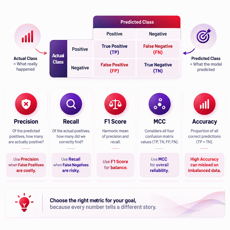
Confusion Matrix Calculator results turn TP, FP, FN, and TN into a clear view of classifier behavior. Instead of trusting accuracy alone, compare precision, recall, F1, error rates, and MCC together. The strongest metric depends on which mistake costs more in your application.
- Use precision when false positive actions are expensive.
- Use recall when missing real positives creates greater risk.
- Use F1 when precision and recall need one balanced summary.
- Use MCC when both classes should influence one score.
- Check class imbalance before trusting a high accuracy value.
- Keep TP, FP, FN, and TN visible during every model comparison.
- Treat undefined metrics as meaningful edge cases, not automatic zeros.
- Reverse solve only when one relevant missing cell is uniquely determined.
A Confusion Matrix Calculator is most useful when its outputs support a real decision. Confirm the positive class, evaluation dataset, and threshold first. Then match the primary metric to the cost of false positives and false negatives. AxiCalculator keeps the calculation fast, while the matrix keeps the interpretation transparent.
Assumptions used in this calculator
- The calculator assumes a binary classification problem with positive and negative classes.
- Input counts represent the same evaluation dataset and classification threshold.
- True positive, false positive, false negative, and true negative values are nonnegative.
- Blank values are treated as unknown, not automatically as zero.
- Fractional counts are assumed to represent intentionally weighted observations.
- Ratio metrics use exact entered values before any display rounding.
- Percentage display changes presentation only, not the underlying metric.
- Undefined denominators produce undefined results instead of misleading zero values.
- Reverse solving assumes exactly one relevant confusion-matrix value is unknown.
- Reverse solutions must be finite, nonnegative, and mathematically consistent.
- MCC reverse solving uses numerical bracketing and bisection when required.
- Model interpretation depends on class balance, threshold, and application costs.
- Results assume supplied labels and predictions are correctly categorized.
Results are rounded for display.
Internal calculations use full precision.
Formulas Used in Confusion Matrix Variables :
TP = true positive count
FP = false positive count
FN = false negative count
TN = true negative count
N = total number of evaluated observations
x = the single unknown confusion-matrix cell during reverse solving
MCC target = manually entered Matthews correlation coefficient used for reverse solving
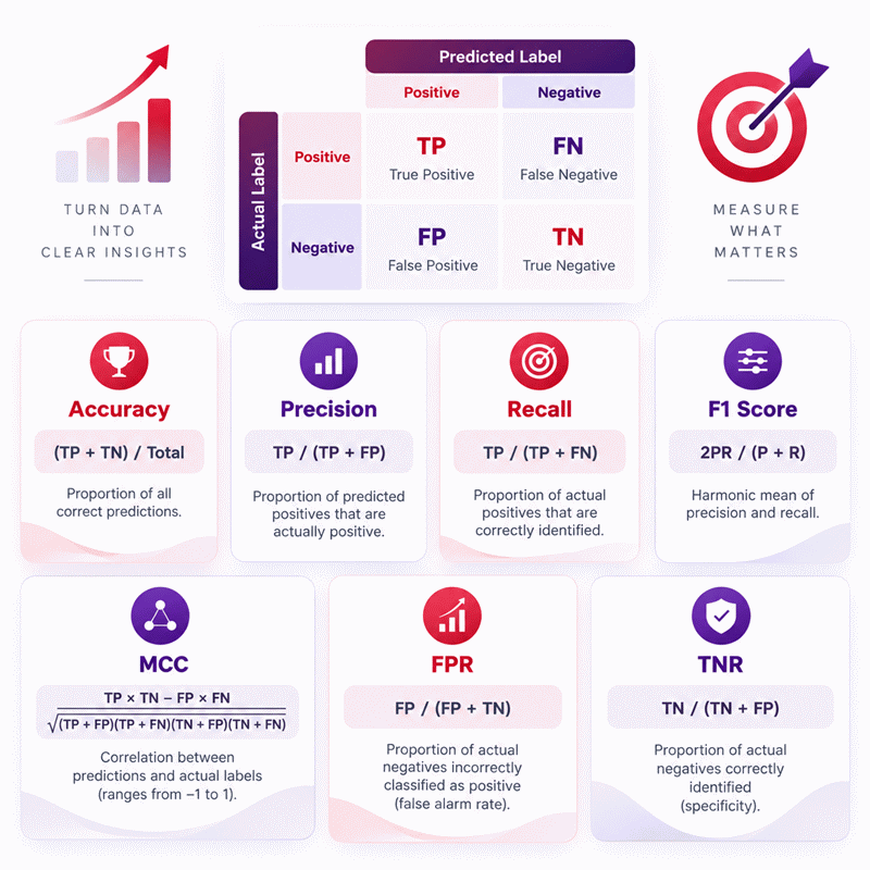
Total observations
Accuracy
Precision and false discovery rate
Recall, true positive rate, and false negative rate
False positive rate and true negative rate
F1 score
Matthews correlation coefficient
Ratio and percentage conversion
Reverse accuracy
Reverse precision
Reverse recall or true positive rate
Reverse false negative rate
Reverse false positive rate
Reverse true negative rate
Reverse false discovery rate
Reverse F1 score
Reverse Matthews correlation coefficient
Variables & Definitions
View a complete list of all variables used in this calculator, including definitions and units
Confusion Matrix Variables and Performance Metrics
| Variable | Name | Valid Range | Unit | Role |
|---|---|---|---|---|
TP |
True positive | 0 or greater | count | Actually positive observations correctly predicted positive. |
FP |
False positive | 0 or greater | count | Actually negative observations incorrectly predicted positive. |
FN |
False negative | 0 or greater | count | Actually positive observations incorrectly predicted negative. |
TN |
True negative | 0 or greater | count | Actually negative observations correctly predicted negative. |
N |
Total observations | Greater than 0 for a complete matrix | count | Sum of TP, FP, FN, and TN. |
Accuracy |
Accuracy | 0 to 1 | ratio or % | Share of all observations classified correctly. |
Precision |
Precision | 0 to 1 | ratio or % | Share of predicted positives that are true positives. |
Recall |
Recall | 0 to 1 | ratio or % | Share of actual positives correctly identified. |
F1 |
F1 score | 0 to 1 | ratio or % | Harmonic balance between precision and recall. |
TPR |
True positive rate | 0 to 1 | ratio or % | Equivalent to recall for binary classification. |
FNR |
False negative rate | 0 to 1 | ratio or % | Share of actual positives incorrectly predicted negative. |
FPR |
False positive rate | 0 to 1 | ratio or % | Share of actual negatives incorrectly predicted positive. |
TNR |
True negative rate | 0 to 1 | ratio or % | Share of actual negatives correctly predicted negative. |
FDR |
False discovery rate | 0 to 1 | ratio or % | Share of predicted positives that are false positives. |
MCC |
Matthews correlation coefficient | -1 to 1 | ratio | Correlation-based measure using all four matrix cells. |
x |
Unknown matrix cell | 0 or greater | count | Single missing TP, FP, FN, or TN value during reverse solving. |
MCC target |
Target MCC | -1 to 1 | ratio | Entered MCC constraint used to numerically recover one unknown cell. |
Unit Conversion Table
Confusion Matrix Count Unit
| Unit Group | Unit Name | Symbol | Equivalent in Base Unit | Used For |
|---|---|---|---|---|
| Observation Count | Count | count | 1 count | TP, FP, FN, TN, and total observations |
Dimensionless Ratio Unit
| Unit Group | Unit Name | Symbol | Equivalent in Base Unit | Used For |
|---|---|---|---|---|
| Dimensionless Metric | Ratio | ratio | 1 ratio | Accuracy, precision, recall, F1, TPR, FNR, FPR, TNR, FDR, and MCC |
Percentage Display Unit
| Unit Group | Unit Name | Symbol | Equivalent in Base Unit | Used For |
|---|---|---|---|---|
| Dimensionless Metric | Percentage | % | 1% = 0.01 ratio | Accuracy, precision, recall, F1, TPR, FNR, FPR, TNR, and FDR |
Example Calculation
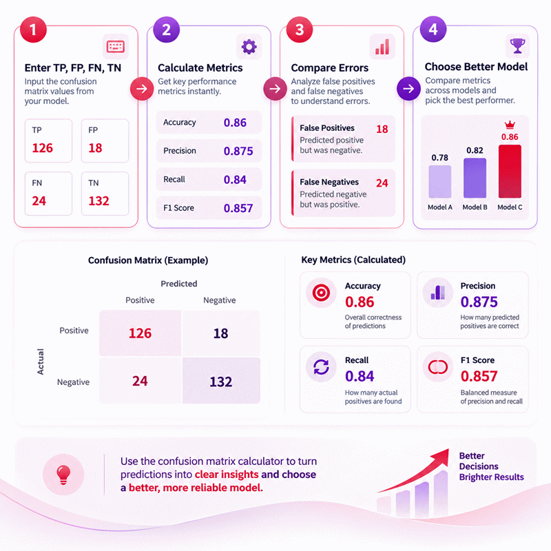
The classifier correctly handles 258 of 300 observations, producing an accuracy of 86%. Precision is 87.5%, while recall is 84%, so positive predictions remain reasonably balanced. The 12% false positive rate and 16% false negative rate expose the remaining classification errors. An MCC of about 0.721 indicates substantial positive agreement across all four matrix cells.
Precision supplies enough information to recover FP because TP is already known. Solving the precision equation produces exactly 18 false positives. The recovered value completes the four-cell confusion matrix and enables every remaining metric. Recalculating precision from TP = 126 and FP = 18 returns 0.875, confirming the reverse solution.
Results are rounded for display.
Internal calculations use full precision.
Calculations Disclaimer
What Does a Confusion Matrix Calculator Reveal That Accuracy Can Hide?
A model can look impressive and still fail where the decision matters. A Confusion Matrix Calculator exposes that risk quickly. It separates correct predictions from two different error types. That separation changes how a score should be trusted.
Accuracy answers one broad question. It tells you how often the classifier was correct overall. That can be useful when both classes are balanced. It can also mislead when one class dominates the dataset. A model may collect many easy negative predictions. Its accuracy then rises, even while positive cases are missed.
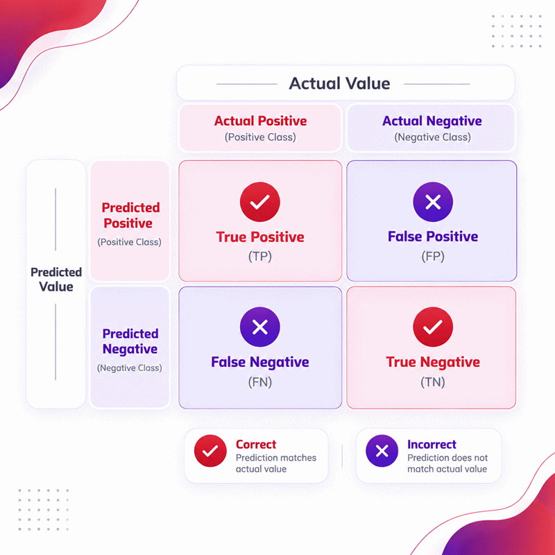
The matrix keeps those failures visible. True positives show successful positive detections. True negatives show successful negative decisions. False positives show false alarms. False negatives show missed positives. Those four outcomes are more informative than one percentage.
This matters because mistakes rarely cost the same. A false alarm may waste review time. A missed positive may cause a larger operational loss. The reverse can also be true. The correct metric therefore depends on the decision.
→ Eye-drag check: If one score looks unusually strong, inspect the two error cells next.
AxiCalculator helps keep that review compact. Enter the known matrix values. Then compare the resulting metrics together. Do not treat one result as a universal verdict. Read the pattern instead.
Why the Four Cells Matter More Than One Headline Score
A reporting dashboard often needs one number. That pressure creates a common mistake. Teams select accuracy because it feels familiar. Yet one number cannot describe every error direction.
The four cells preserve context. A rise in false positives damages precision. A rise in false negatives damages recall. Both can happen while overall accuracy changes only slightly. That is why the underlying counts should stay visible.
Think of the matrix as an audit trail. It shows what the model did. Metrics then summarize different parts of that behavior. A good review starts with the cells. It does not start with a preferred score.
This structure also makes model comparison safer. Two classifiers can share similar accuracy. Their operational behavior may be completely different. One may generate many false alarms. Another may miss important positives. Those models should not be treated as equivalent.
Spot False Alarms and Missed Positives Before They Become Decisions
The fastest practical check is simple. Ask which error creates the larger consequence. If false positives cause unnecessary action, inspect precision and false positive behavior. If false negatives create the larger risk, inspect recall and false negative behavior.
This question should come before optimization. Otherwise, a team may improve the wrong metric. A higher score can still produce a worse business outcome. The model is useful only when its errors match the acceptable risk.
Text infographic: Prediction review → Identify costly error → Choose matching metric → Compare supporting metrics → Decide.
How Should You Read TP, FP, FN, and TN Without Mixing Them Up?
Many reporting errors begin before any metric is calculated. The positive class gets changed, or the axes get reversed. The numbers still look valid. Their meaning does not.
Start by fixing the positive class. The positive class is the event you want to detect. It might be fraud, spam, a defect, or another target event. Once that class is fixed, every cell has a stable meaning.
A true positive is a positive case predicted positive. A false positive is a negative case predicted positive. A false negative is a positive case predicted negative. A true negative is a negative case predicted negative.
The words “false positive” and “false negative” describe error direction. They are not interchangeable labels. A false positive is a false alarm. A false negative is a miss. That distinction should stay visible in every report.
When data comes from another system, inspect its row and column convention. Some libraries place actual labels on rows. Others may present predicted labels first. Never assume the location of TP from the visual position alone.
Lock the Positive Class Before Interpreting Any Metric
Positive does not mean good. It means the class treated as the target event. This distinction prevents serious interpretation mistakes.
Consider a safety classifier. “Positive” might mean a dangerous condition exists. In another workflow, “positive” might mean a transaction is approved. The same metric name can carry very different practical meaning.
Changing the positive class changes precision and recall. It also changes TPR, FNR, FPR, and TNR interpretation. A model review should therefore state the positive class clearly before discussing performance.
A reliable report also uses one evaluation population. Mixing counts from different periods breaks the matrix. The totals may still add correctly, but the metrics no longer describe one coherent test.
Use Error Direction to Understand What the Model Actually Gets Wrong
Error direction often reveals more than overall error volume. Many false positives suggest the model fires too easily. Many false negatives suggest the model is too conservative. The next action depends on that direction.
Do not reduce this to “higher is better.” A better model aligns its errors with real operating costs. That may require accepting more of one error type to reduce another.
→ Eye-drag check: Name the positive class aloud before trusting any precision or recall value.
Which Metric Should You Trust When the Scores Disagree?
Conflicting metrics are not a calculator problem. They are information. Each metric asks a different question. Disagreement shows that the classifier behaves differently across parts of the matrix.
Accuracy summarizes total correctness. Precision checks the reliability of positive predictions. Recall checks how many actual positives were found. F1 balances precision and recall. MCC evaluates agreement using all four cells.
There is no universal winner. The correct metric follows the decision cost. A fraud review team may dislike false positives because they block legitimate users. A safety team may dislike false negatives because missed hazards are costly. The same classifier can be judged differently under those goals.
Start with the costliest error. Then choose the primary metric. Use at least one supporting metric to prevent tunnel vision. The raw matrix should remain available during the decision.
Choose Accuracy Only When the Class Balance Makes It Meaningful
Accuracy is easiest to explain. That makes it attractive. It is also the score most likely to be overused.
Accuracy works best when class sizes are reasonably balanced. It is also more useful when the two error types have similar costs. If either condition fails, accuracy needs support from other metrics.
A highly imbalanced dataset creates a familiar trap. The majority class can dominate the score. A model may look excellent because it predicts the common class well. The rare class can still be handled poorly.
Use accuracy as a summary, not a shield. If the positive class is rare, always inspect recall and precision. If both classes must influence one summary score, inspect MCC as well.
Use Precision When False Positives Create the Bigger Cost
Precision answers a direct operational question. When the model predicts positive, how often is that prediction right?
Low precision means too many positive predictions are false alarms. That can waste human review. It can also create unnecessary interventions. In customer-facing systems, false alarms may reduce trust.
High precision is valuable when positive actions are expensive. It does not prove that most positives were found. A conservative model can achieve high precision while missing many real positives.
Use Recall When Missing Positives Creates the Bigger Risk
Recall focuses on actual positives. It asks how many were successfully detected.
Low recall means important positives are being missed. That matters in detection workflows. It also matters when delayed discovery is costly.
High recall can increase false alarms. That trade-off may be acceptable. The answer depends on the real consequence of missing a positive case.
Why Can F1 and MCC Tell Different Stories About the Same Classifier?
A team may expect F1 and MCC to move together. Often they do. Sometimes they do not. That disagreement is useful.
F1 focuses on the positive class. It combines precision and recall. True negatives do not directly control its value. That makes F1 useful when positive-class performance is the main concern.
MCC behaves differently. It uses information from all four cells. This gives both classes influence over the summary. A model that performs unevenly across classes may therefore receive a different MCC story.
Neither score should be treated as magical. F1 is focused. MCC is broader. Choose the score that matches the evaluation goal.
When the values disagree, return to the matrix. Inspect the negative-class behavior. Then inspect class balance. The reason is usually visible there.
Understand What F1 Ignores Before Making a Model Decision
F1 is often praised for class-imbalanced problems. That description needs context. F1 protects you from some accuracy problems. It does not inspect true negatives directly.
This can be an advantage. A huge negative class will not dominate F1. It can also be a limitation. A system may care deeply about correctly clearing negative cases.
Use F1 when positive predictions and missed positives deserve balanced attention. Do not use it alone when negative-class behavior affects real decisions.
Also remember that identical F1 values can hide different trade-offs. One model can have higher precision. Another can have higher recall. Their practical behavior can differ.
Use MCC When Both Classes Must Influence One Summary Score
MCC provides a correlation-style view of binary prediction quality. It considers the full matrix. That makes it useful when neither class should dominate the evaluation.
A positive MCC indicates useful alignment. A value near zero suggests weak association. A negative value signals inverse behavior. The number becomes most useful when paired with the matrix.
MCC can also become undefined in edge cases. That is not a reason to force a zero. Undefined output tells you the matrix lacks the variation needed for that calculation.
A trustworthy calculator should preserve this state. A made-up zero would change the meaning. AxiCalculator keeps undefined conditions separate from genuine zero performance.
How Does Class Imbalance Change the Meaning of a Good Result?
A model can score well because the dataset is easy in one direction. Class imbalance creates that illusion. The majority class produces many opportunities for easy correct predictions.
Suppose the negative class dominates. The classifier may learn to predict negative often. True negatives rise quickly. Accuracy follows. Yet the model may fail on the minority positives.
This is why “good” has no fixed numeric meaning. A score only makes sense within the class distribution and operating goal. Compare models on the same evaluation population whenever possible.
When datasets differ, first inspect prevalence and error counts. A score can change because the population changed. The model itself may not have improved or worsened.
Text infographic: Class balance → Error pattern → Metric sensitivity → Operational cost → Final interpretation.
Detect the Accuracy Trap Before It Misleads a Report
The accuracy trap is easy to recognize. One class dominates. Accuracy looks excellent. Minority-class recall looks weak.
A report should flag that pattern immediately. Do not hide it behind an average. Show the four matrix cells and at least one minority-sensitive metric.
Also compare the classifier against a simple baseline. If always predicting the majority class produces similar accuracy, the headline score has little value.
This check is especially important in rare-event systems. Fraud, faults, abuse, and anomaly detection often contain few positives. Those are exactly the situations where accuracy needs caution.
Read Minority-Class Errors Before Celebrating a High Score
A minority class can contain the most valuable cases. Its small size does not reduce its importance. The cost of missing it may be large.
Check false negatives first when detection matters. Check false positives first when intervention cost matters. Then compare the supporting metric.
→ Eye-drag check: A 99% headline score deserves more inspection, not less.
How Do Threshold Changes Reshape Precision, Recall, FPR, and FNR?
A confusion matrix describes one decision rule. Many classifiers start with a score or probability. A threshold converts that score into a class label.
Move the threshold and the matrix changes. A lower threshold usually creates more positive predictions. That can increase true positives. It can also increase false positives.
A higher threshold usually makes positive predictions harder. False positives may fall. False negatives may rise. Precision and recall then move in opposite directions.
This trade-off is not a defect. It is the heart of classification decisions. The best threshold depends on the cost of each error.
Do not compare thresholds using one metric blindly. Track the metric tied to the decision. Also watch the supporting error rate. This prevents hidden damage elsewhere.
Connect Every Threshold Move to a Real Error Trade-Off
A threshold should never be tuned only for a prettier dashboard. It should connect to a real outcome.
If reviewing a false alarm costs minutes, quantify that burden. If missing a positive causes a larger loss, quantify that risk. The threshold can then reflect actual priorities.
Document the chosen threshold with the evaluation dataset. Otherwise, future teams may reproduce the model but not the decision behavior.
A confusion matrix should be regenerated after threshold changes. Old metrics no longer describe the current operating point.
Can You Reverse Solve a Missing Confusion Matrix Value?
Reports often arrive incomplete. A metric may be known while one matrix cell is missing. Reverse solving can recover that cell in some cases.
The key word is “some.” A metric only contains information about specific cells. Precision, for instance, depends on positive predictions. It cannot determine an unrelated missing true-negative value.
A reliable reverse solver checks dependency first. It then checks uniqueness. If the known values cannot determine one answer, the calculator should refuse to guess.
This behavior is useful during audits. You can test whether a reported metric agrees with the available counts. You can also recover one missing value when the relationship is sufficient.
Reverse solving should preserve the original metric as a constraint. It should never silently rewrite an arbitrary input to make the numbers fit.
Know When One Metric Determines the Missing Cell Uniquely
A reverse solution is strongest when exactly one relevant cell is unknown. The selected metric must depend on that cell. The remaining required values must be known.
Boundary values need extra care. A metric at zero or one can create several valid solutions. It can also create no valid solution. The calculator must distinguish those outcomes.
Numeric solving may be needed for more complex metrics. The result still needs verification. A solved cell should reproduce the entered target metric within a tight tolerance.
This approach turns reverse solving into an audit tool. It is not merely a convenience feature.
Avoid Reverse Solutions When the Information Is Insufficient
Guessing a missing cell creates false confidence. A professional tool should show insufficiency clearly.
If two matrix cells are missing, one metric usually cannot identify both. If the metric ignores the missing cell, no reverse solution exists. If several answers fit, the solution is not unique.
The safe response is explicit. Ask for more information. Do not choose a value because it looks reasonable.
What Should You Check Before Using Confusion Matrix Results in Practice?
A mathematically correct result can still support a bad decision. The evaluation setup matters as much as the arithmetic.
First, verify the labels. Confirm the positive class. Confirm the row and column convention. Then verify that every count belongs to the same test population.
Next, inspect class balance. A representative sample matters. If deployment data differs sharply, the reported metrics may not transfer cleanly.
Then inspect the threshold. Metrics calculated at one threshold do not describe another threshold. Record the operating point used during evaluation.
Finally, connect metrics to cost. A model with fewer false positives may save review time. A model with fewer false negatives may reduce missed events. The preferred model depends on that trade-off.
AxiCalculator can accelerate the arithmetic. The final decision still belongs to the evaluation context.
Audit Labels, Dataset Shift, Sample Size, and Decision Costs
Label quality comes first. Incorrect ground truth corrupts every cell. A perfect formula cannot repair bad labels.
Dataset shift comes next. A model tested on one population may face another population later. Class prevalence can change. Input patterns can change. Error rates can change with them.
Sample size also affects confidence. A metric calculated from a tiny number of cases can move sharply after one new observation. Treat small tests cautiously.
Decision cost turns statistics into action. Write down what each error means operationally. This makes metric selection defensible.
Turn Calculator Outputs Into a Defensible Model Review
A strong review is easy to reconstruct. It records the matrix counts, positive class, dataset, threshold, and selected metrics. It explains why those metrics matter.
Keep the raw matrix beside the summary. Report the primary metric and at least one supporting metric. Note undefined values instead of hiding them.
When comparing models, use the same evaluation population. Keep the same label convention. Keep the same threshold logic unless threshold tuning is the comparison itself.
That process creates a review others can challenge and reproduce. It also reduces the chance of choosing a model because one headline score looked attractive.
Use AxiCalculator as the fast calculation layer. Use your domain knowledge as the decision layer. The combination is more reliable than either one alone.
Frequently Asked Questions
Why can two classifiers with similar accuracy behave very differently?
What should I do when precision and recall move in opposite directions?
Why does changing the positive class change my interpretation?
Should I report percentages or ratios for confusion-matrix metrics?
How should an engineer validate a reverse-solved confusion-matrix cell?
What does an undefined MCC indicate during a model audit?
How can dataset shift make an old confusion matrix unreliable?
Our engineers are here to help you get it right.