Chebyshev’s Theorem Calculator

Last formula update: September 22, 2026

Trusted Engineering Tools

Use the Chebyshev’s Theorem Calculator to turn uncertain distribution shape into a clear, conservative probability bound. Enter the values you know, solve missing parameters in either direction, and understand exactly what your data can guarantee.

Formula

P(|X - E(X)| ≥ k) ≤ variance / k^2

P(|X - E(X)| ≥ k * sigma) ≤ 1 / k^2

Formula parameters At least two independent values are required.

Bound (k)

Variance (sigma^2)

Divergence

Probability

Results

Maximum divergence probability

Minimum within bound

Divergence threshold

Decimal & Rounding Policy

All calculations retain full available precision before final display formatting.
Intermediate variance, divergence, bound, and probability values are never rounded early.
Probability ratios use decimal form internally, where 0.15 equals 15%.
Displayed results use up to 10 significant digits when additional precision is meaningful.
Automatically back-solved editable values retain up to 12 significant digits.
Probability bounds above 100% are limited to 100% in reported probability results.
Rounding affects display only and never changes the underlying Chebyshev calculation.

Valid range

Bound k must be finite and greater than 0.
Variance must be finite and nonnegative in the absolute-bound form.
Variance must be finite and greater than 0 in the standardized form.
Divergence must be finite and greater than 0 when entered directly.
The raw Chebyshev bound ratio must be finite and nonnegative.
A raw bound above 1 is mathematically valid but gives only a trivial probability bound.
Reported event probability is limited to the physical range from 0 to 1.
Percentage probability therefore ranges from 0% to 100% after probability capping.
Reverse solving requires a positive bound ratio when solving for a finite positive k.
For a useful standardized inside-range guarantee, k should normally be greater than 1.

Creators

Wylena Brantford

Reviewers:

Valdren Clyforde

Zenara Dentwick

Check our editorial policy

Formula Implementation date:

September 22, 2026

Formula Version:

1.0.0

Changelog:

Version 1.0.0

Initial calculator and formula release.

Need help selecting or validating calculations?

Our engineers are here to help you get it right.

What Can a Chebyshev’s Theorem Calculator Guarantee About Your Data?

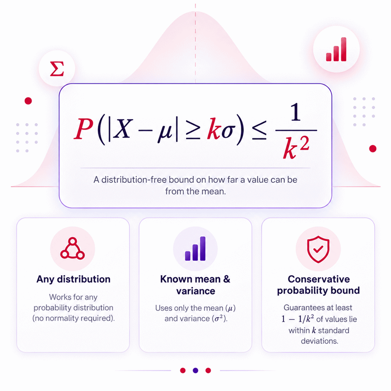
Chebyshev’s Theorem Calculator gives a distribution-free probability bound when the exact shape of your data is unknown. It shows the maximum probability of observations lying far from the mean and the guaranteed minimum probability remaining within a selected distance.

The result is a mathematical guarantee, not an exact observed percentage.
It can be used with skewed, asymmetric, bimodal, or otherwise non-normal distributions.
A larger distance from the mean produces a stronger guaranteed coverage.
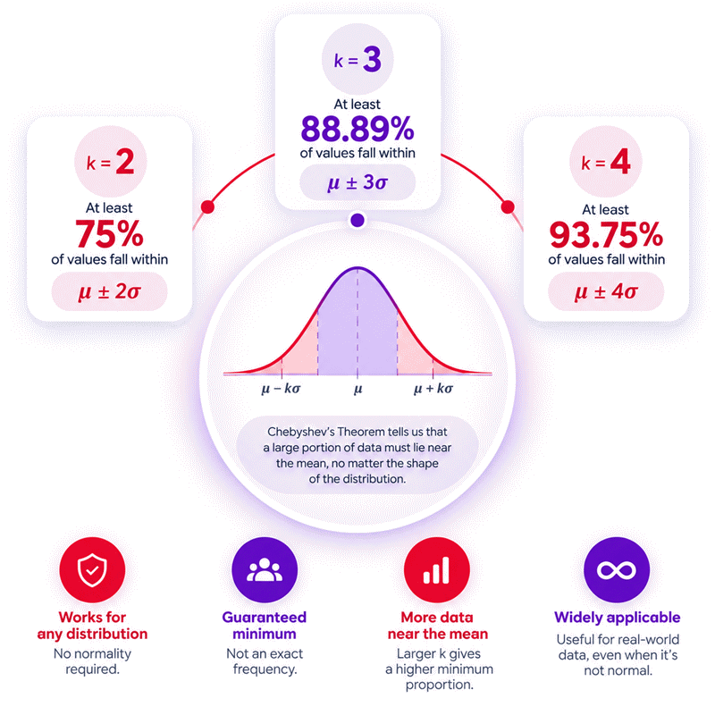
Two standard deviations guarantee at least 75% inside the interval.
Three standard deviations guarantee at least about 88.89% inside.
Weak or trivial bounds indicate that available information is insufficient for a stronger universal conclusion.
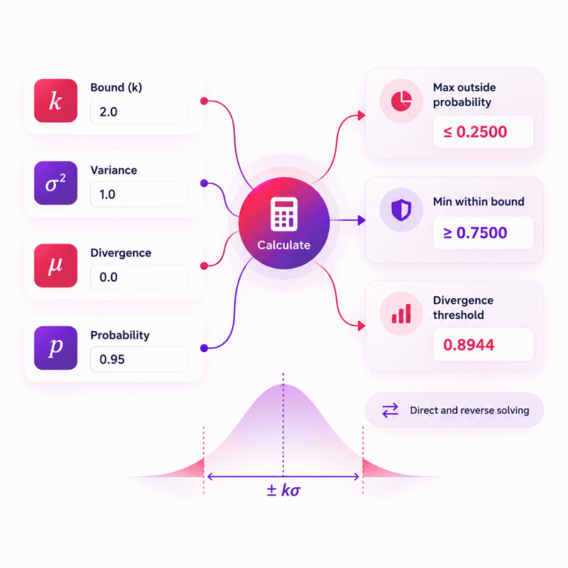
Reverse solving can recover a missing bound, divergence, variance, or probability when enough independent information is available.

The Chebyshev’s Theorem Calculator is most useful when you need a conservative baseline without assuming a normal distribution. Treat its output as a worst-case guarantee, then compare it with observed data or a stronger statistical model when reliable distribution information is available.

Assumptions used in this calculator

The random variable has a finite expected value and finite variance.
Variance is expressed in squared units of the random variable.
Bound values are strictly positive whenever used as calculation inputs.
Standardized calculations use a positive, finite standard deviation.
No normal distribution assumption is required for Chebyshev bounds.
Probability outputs are bounds, not exact event probabilities.
Bounds above one are limited to one hundred percent when reported.
Reverse solving treats entered probability as the Chebyshev upper bound.
Divergence uses the same base unit as the random variable.
Input units remain dimensionally consistent throughout each calculation.
Intermediate calculations retain full available numerical precision.
Displayed rounding does not alter the underlying calculation.
Extreme values may be limited by browser floating-point precision.

Results are rounded for display.
Internal calculations use full precision.

Formulas Used in Chebyshev's Theorem Calculator :

Absolute Chebyshev Bound

P(|X − μ| ≥ k) ≤ b , b = σ² k²

Standardized Chebyshev Bound

P(|X − μ| ≥ kσ) ≤ b , b = 1 k²

Divergence Threshold

d = kabsolute form kσstandardized form

Reported Probability Bounds

p_out = min(1, b) , p_in = 1 − p_out

Variables

X = random variable.
μ = E(X), the expected value of X.
σ² = finite variance of X.
σ = standard deviation, equal to the square root of variance.
k = positive bound parameter.
d = actual divergence threshold measured in the units of X.
b = raw Chebyshev upper-bound ratio.
p_out = reported maximum probability outside the threshold.
p_in = guaranteed minimum probability inside the threshold.

Variables & Definitions

View a complete list of all variables used in this calculator, including definitions and units

Chebyshev's Theorem Calculator Variables and Symbols

Variable	Meaning	Calculation Role	Valid Range	Unit
X	Random variable being analyzed	Defines the uncertain quantity around its expected value	Depends on the modeled process	Base variable unit
μ	Expected value E(X)	Center point from which divergence is measured	Any finite value supported by X	Same as X
σ²	Variance of X	Measures dispersion used in the absolute Chebyshev bound	≥ 0 and finite; > 0 for standardized solving	Base unit squared
σ	Standard deviation of X	Converts a standardized k value into actual divergence	≥ 0; positive in standardized calculations	Same as X
k	Chebyshev bound parameter	Sets the distance from the expected value	> 0	Base unit or SD multiplier
d	Divergence threshold	Actual distance from the expected value	> 0	Same as X
b	Raw Chebyshev upper-bound ratio	Provides the mathematical upper bound before probability capping	≥ 0 and finite	Dimensionless
p_out	Reported maximum outside probability	Limits the raw bound to a valid probability	0 to 1	Decimal or %
p_in	Guaranteed minimum inside probability	Complements the reported outside probability	0 to 1	Decimal or %

Unit Conversion Table

Chebyshev's Theorem Calculator Unit Conversion Table

Unit Group	Unit Name	Symbol	Equivalent in Base Representation	Used For
Distance	Base Random-Variable Unit	u	1 u	Absolute bound and divergence threshold
Variance	Squared Base Unit	u²	1 u²	Variance of the random variable
Standardized Distance	Standard Deviation	SD	1 SD = σ u	Standardized bound k and divergence calculation
Probability	Percent	%	1% = 0.01	Probability bound input and result display
Probability	Decimal Probability	decimal	1 = 100%	Internal probability calculations and reverse solving

Example Calculation

Variance 14.4 u²

Bound k 6 u

b = σ² k² = 14.4 6² = 14.4 36 = 0.4

P(|X − μ| ≥ 6) ≤ 0.4 = 40%

p_in = 1 − 0.4 = 0.6 = 60%

Maximum probability outside the 6 u divergence threshold: 40%
Minimum probability within 6 u of the expected value: 60%
Divergence threshold: 6 u

A process with variance 14.4 u² is evaluated at a 6 u distance from its expected value.

Chebyshev's inequality limits the probability outside that distance to at most 40%.

Therefore, at least 60% of observations are guaranteed to remain within the selected distance.

The actual inside proportion may be higher because the theorem provides a conservative bound.

Probability upper bound 16%

Variance 25 u²

σ = √ 25 = 5 u

k = 1 √ 0.16 = 1 0.4 = 2.5

d = kσ = 2.5 × 5 = 12.5 u

p_in = 1 − 0.16 = 0.84 = 84%

Back-solved bound k: 2.5 SD
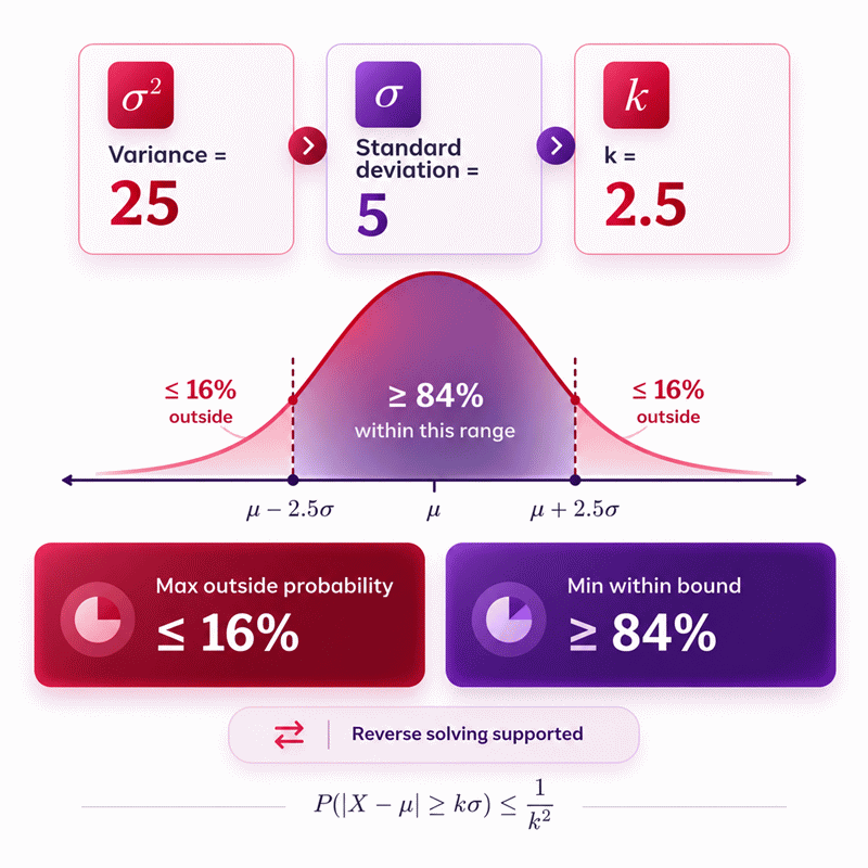
Back-solved standard deviation: 5 u
Divergence threshold: 12.5 u
Minimum probability within the threshold: 84%

The calculation starts with a 16% Chebyshev upper bound and variance of 25 u².

Reverse solving gives a bound of 2.5 standard deviations from the expected value.

Because the standard deviation is 5 u, the corresponding divergence is 12.5 u.

At least 84% of observations are therefore guaranteed within that divergence threshold.

Results are rounded for display.
Internal calculations use full precision.

Calculations Disclaimer

Read important information about accuracy, limitations and responsible use of this calculator

Chebyshev’s Theorem Calculator provides mathematical probability bounds based on the entered variance and distance from the expected value. The result is an upper or lower guarantee derived from Chebyshev’s inequality, not an exact probability forecast. The method requires a random variable with a finite expected value and finite variance, but it does not require a normal distribution. Chebyshev bounds can be conservative, especially when little is known about the underlying distribution. A calculated raw bound above 100% is mathematically valid as an inequality but provides only the trivial probability limit of 100%. Results should be interpreted as statistical bounds and should not replace application-specific risk analysis, experimental validation, or professional judgment.

What Does a Chebyshev’s Theorem Calculator Actually Tell You?

A dataset can look stable until one extreme observation changes the decision. That problem becomes harder when nobody can justify a normal distribution. A Chebyshev’s Theorem Calculator gives a conservative answer without forcing that assumption. It tells you how much probability can remain far from the mean. It can also show how much must stay within a selected distance.

The key word is guarantee. The result does not claim that your dataset contains exactly the displayed percentage. Instead, it gives a mathematical floor or ceiling. That distinction matters in quality control, financial risk, reliability work, laboratory analysis, and statistics coursework. A result of 75% within a selected interval does not mean exactly 75% will appear there. It means the true proportion cannot fall below that guarantee under the stated statistical conditions.

This makes the calculator useful when information is limited. You may know the center and variability of a process. You may not know its complete distribution. A narrow model could create false confidence. A distribution-free result gives a safer baseline.

Decision path: Unknown distribution shape → known variability → choose a distance → read the guaranteed bound.

The outside result deserves equal attention. It represents a maximum permitted probability beyond the selected distance. The inside result is its conservative complement. Reading both values prevents a common error. Users often see one percentage and treat it as an exact frequency. That interpretation is too strong.

AxiCalculator keeps these ideas separate. The interface lets you work from known parameters or reverse the problem. This is useful when your question begins with a target rather than a known distance. You may know how much outside risk you can tolerate. The missing quantity may be the distance needed to achieve that bound.

The result should therefore answer a decision question, not merely produce a number. Ask whether you need a guaranteed floor, a predicted probability, or an observed sample percentage. Chebyshev addresses the first question. It does not automatically answer the other two.

Why a Guaranteed Minimum Is Different From an Exact Probability

A manager sees “at least 84%” and reports “84% of our measurements are inside.” That change looks small, but it changes the scientific meaning. A guarantee is a lower limit. Actual coverage can be higher.

Imagine two processes with identical means and variances. Their shapes can still differ greatly. One may place most observations close to the center. Another may spread probability more aggressively. A distribution-free bound must remain valid for both. That is why it can look conservative.

This conservatism is not a defect. It is the price of using fewer assumptions. When a stronger distribution model is justified, a tighter answer may be available. When the shape is unknown, a universal guarantee can be more defensible.

How to Read Maximum Outside Probability Without Overstating Risk

A risk analyst may see a maximum outside probability of 16% and call the event “16% likely.” That statement is not justified. The number is a ceiling supplied by the inequality.

The actual outside probability may be 16%, 8%, 2%, or another smaller value. The calculator does not infer the exact tail shape. It limits what the probability can be under the available information.

Use wording such as “at most,” “no greater than,” or “bounded above by.” Those phrases preserve the statistical meaning. They also make reports easier to audit.

When Should You Use Chebyshev’s Inequality Instead of a Distribution Model?

A production engineer receives a month of irregular measurements. The histogram is skewed, and a normality assumption looks doubtful. The team still needs a defensible statement about dispersion. This is a strong use case for a distribution-free bound.

Chebyshev is valuable when you trust the basic measures of center and variability more than you trust a particular distribution shape. It does not require the curve to look symmetric. It does not require a bell shape. It remains useful when data is lopsided or multimodal.

That flexibility creates a practical hierarchy. First ask what you actually know. If a distribution model is well supported, use its stronger information. If the shape is uncertain, avoid pretending otherwise. A conservative universal bound can be the more responsible answer.

This distinction is important in early-stage analysis. Teams often have enough observations to estimate variability but not enough evidence to defend a detailed probability model. A model-specific result may look precise while resting on a weak assumption. Chebyshev makes that uncertainty visible.

DATA SHAPE KNOWN AND JUSTIFIED → consider a model-specific probability method
DATA SHAPE UNKNOWN, VARIABILITY AVAILABLE → use a distribution-free Chebyshev bound
NO RELIABLE VARIABILITY → do not force a Chebyshev conclusion

The calculator is also valuable as a reasonableness check. Suppose another method produces an aggressive probability statement. A conservative bound gives you a second perspective. The two numbers answer different questions, but the contrast can expose an assumption that deserves review.

AxiCalculator is most useful when the analyst treats the output as evidence, not authority. The calculator reduces arithmetic effort. It does not remove the need to understand the data-generating process.

What Changes When Your Data Is Skewed, Bimodal, or Unknown?

A skewed process often breaks intuitive expectations. Most observations may cluster on one side while a long tail stretches on the other. A bimodal process can have two strong clusters. A normal approximation can miss both structures.

Chebyshev avoids that shape assumption. Its guarantee is deliberately broad enough to survive those cases. This is why the result may appear looser than a familiar normal-distribution percentage.

The advantage is reliability across shapes. The disadvantage is reduced sharpness. You trade precision for robustness.

Why Finite Variability Matters More Than Distribution Shape

A dataset can have an unusual shape and still support a Chebyshev analysis. The more serious problem appears when the required variability measure is not finite or not meaningful.

Before using the result, confirm that your data and statistical model support a stable variance. Extreme heavy-tail behavior can make this assumption inappropriate. The calculator cannot repair a poor statistical description.

This check is especially important when data comes from unstable processes, rare-event systems, or incomplete sampling.

How Does Distance From the Mean Change the Probability Guarantee?

A quality team widens an acceptable monitoring band and notices the guaranteed coverage rises quickly. That behavior is central to Chebyshev analysis. Farther thresholds permit a stronger statement about how much probability must remain inside.

This does not mean wider limits improve the process. The process has not changed. Only the question changed. You are asking how much data is guaranteed within a larger region.

That difference prevents a dangerous interpretation. A wide interval can create an impressive coverage percentage while being operationally useless. A tolerance band and a statistical guarantee are not automatically the same thing.

Use the calculator in two stages. First choose a distance that matters to the real decision. Then evaluate the guarantee. Do not choose a large distance merely to obtain a pleasing percentage.

Wider interval ≠ better process.
Wider interval = easier coverage guarantee.

This matters in engineering and quality systems. A component may need to remain inside a narrow functional tolerance. A broad statistical interval cannot replace that specification. Likewise, a financial risk limit cannot be widened simply because the resulting probability bound looks safer.

Chebyshev gives mathematical context. Operational limits still come from the problem itself.

Why Two Standard Deviations Creates a 75 Percent Guarantee

A student often expects two standard deviations to imply roughly 95% because that number is familiar. That expectation belongs to a different assumption set.

With a distribution-free guarantee, two standard deviations provide a weaker floor. The result protects against many shapes, including highly non-normal ones. That wider applicability explains the smaller guaranteed percentage.

Read the result as a safety baseline. If the data later proves close to a specific distribution, a more informative model may be appropriate.

What Three Standard Deviations Really Guarantees

A report may describe three standard deviations as almost complete coverage. That wording can be misleading without a distribution assumption.

Chebyshev still provides a strong minimum guarantee at that distance, but it is not the same as the familiar percentage associated with a normal curve. The calculator keeps the distribution-free interpretation intact.

This is particularly useful when auditability matters. A conservative statement is easier to defend than an unsupported exact-looking percentage.

Why Wider Intervals Improve the Worst-Case Bound Quickly

A user increases the selected distance a little and sees a noticeable reduction in the allowed outside probability. This happens because the relationship changes with the square of distance.

The practical message is simple. Large deviations become progressively harder to accommodate under a fixed variance. That is why the outside ceiling falls quickly as the distance grows.

However, always judge the distance against the real system. Mathematical comfort should not replace an operational requirement.

How Should You Interpret Chebyshev Results in Real Decisions?

A dashboard can show a clean percentage while the underlying business question remains unresolved. The correct interpretation begins by asking what decision the percentage supports.

For risk screening, the result can provide a conservative ceiling on extreme deviations. For quality work, it can show a guaranteed minimum concentration around the mean. For education, it demonstrates what can be concluded without assuming normality. For data analysis, it can act as a baseline against stronger models.

These uses share one rule: do not convert a bound into a forecast. A bound describes what cannot be exceeded or what must be achieved under the stated conditions. A forecast tries to describe what will actually happen.

The calculator can also help prioritize investigation. Suppose the guaranteed coverage is too weak for a decision. That does not necessarily mean the process is poor. It may mean you need more information. You might examine the actual distribution, calculate empirical coverage, test a justified model, or collect more representative data.

BOUND TOO WEAK?
1. Check the chosen distance.
2. Check the variance quality.
3. Inspect the observed distribution.
4. Decide whether a stronger model is justified.
5. Keep the conservative bound as a reference.

This sequence prevents false precision. It also makes the result more useful. Instead of asking whether Chebyshev is “good” or “bad,” ask whether its level of information matches your decision.

AxiCalculator supports that workflow by making the numerical relationship editable. You can explore how a target changes when distance, variability, or probability constraints change. That interactive view often reveals trade-offs faster than a static formula.

Why the Bound Should Be Read as a Safety Floor

A team wants a minimum level of confidence before proceeding. That is exactly where a floor is useful.

If the calculated minimum inside coverage meets the decision threshold, the available information supports that conservative statement. If it does not, the calculation warns that stronger claims require more evidence.

This makes the result valuable in preliminary screening and robust reporting.

What a Conservative Result Can and Cannot Prove

A conservative result can prove a minimum or maximum bound under its mathematical conditions. It cannot reveal the actual histogram, detect process shifts, or prove normality.

It also cannot explain why variance is high. That question requires domain knowledge and data investigation.

Use the calculator to answer the bound question cleanly. Use other statistical tools for diagnosis.

Why Actual Data May Be Much More Concentrated

A dataset can place nearly all observations close to its mean even when Chebyshev promises much less. That is normal behavior for a universal bound.

The theorem must remain correct for difficult distributions. It therefore cannot assume your particular dataset is friendly.

The gap between guaranteed coverage and observed coverage is information. It tells you how much additional structure your real data may possess.

When Does Chebyshev Become Too Conservative to Be Useful?

A user enters a small distance and receives a result that says almost nothing. The calculator is not failing. The selected threshold simply does not allow a useful universal guarantee.

This situation is most obvious near one standard deviation. A distribution-free method must allow a wide variety of probability shapes. At short distances, the worst-case scenario can be too broad to provide an informative inside guarantee.

The correct response is not to manipulate the input. Instead, reconsider the question. Perhaps your operational threshold really is narrow. In that case, Chebyshev may not provide enough information. You may need observed data or a justified distribution model.

A second warning appears when a raw outside bound exceeds the probability ceiling. The inequality can still be mathematically true, but it adds no practical information beyond the fact that probability cannot exceed 100%.

This is a useful diagnostic. It tells you that the available variance and chosen distance are insufficient for a stronger distribution-free conclusion.

A weak bound is not a calculation error.
It is a message: the available information is too limited for a stronger guarantee.

This interpretation protects against overconfidence. Analysts sometimes hide weak results because they appear unhelpful. In reality, knowing that the data cannot support a strong claim is valuable information.

What Happens Near One Standard Deviation?

A student expects every standard-deviation interval to produce a meaningful percentage. That is not the case for a universal bound.

Near one standard deviation, the guarantee becomes weak. The result should be treated as a limitation of the available information, not as evidence that observations are widely dispersed.

If your decision depends on such a narrow region, inspect the actual distribution instead.

Why an Upper Bound Can Become Trivial

A probability calculation returns a mathematical ceiling larger than the largest possible probability. This looks strange until you separate the inequality from the probability scale.

The inequality may still be valid. It simply fails to improve on the obvious statement that probability cannot exceed one.

A well-designed calculator should communicate this rather than presenting an impossible practical probability.

How to Recognize a Result That Adds No Practical Information

If the outside limit effectively reduces to 100%, the result is trivial. If the guaranteed inside proportion reduces to zero, the same problem appears from the opposite direction.

That result should prompt a new analytical step. Increase information quality, inspect the distribution, or use a method suited to the known data structure.

How Does Reverse Solving Change the Way You Use Chebyshev’s Theorem?

An analyst knows the maximum outside risk the project can tolerate but does not know the required distance. A one-way calculator forces manual algebra. Reverse solving starts from the actual decision instead.

This changes the tool from a formula evaluator into a constraint solver. You can enter the quantities you know and allow the missing value to update automatically. That is especially useful during design, planning, and sensitivity analysis.

Consider the decision sequence. A conventional question asks, “Given this distance, what is the bound?” A reverse question asks, “Given this acceptable bound, how far from the mean must the threshold be?” Both belong to the same mathematical relationship, but they support different workflows.

Reverse solving also helps audit existing reports. If someone presents a probability bound and variance, you can recover the implied distance and check whether it matches the documented threshold. If someone presents a distance and bound, you can recover the implied variability and compare it with the dataset.

This makes inconsistency easier to detect. A set of values that cannot describe one coherent relationship should not be silently accepted.

AxiCalculator treats calculated outputs as editable quantities. That design is especially useful for technical users because it avoids duplicating the same variable as separate “input” and “output” controls.

Finding a Required Distance From a Target Probability

A risk limit is often specified first. The analyst then needs to determine how wide a threshold must be before the distribution-free bound satisfies that limit.

Reverse solving handles that workflow directly. As the acceptable outside probability becomes smaller, the required distance grows.

The result should still be checked against operational reality. A mathematically sufficient distance may be too wide for the actual application.

Recovering Variability From a Known Probability Bound

A report may provide a threshold and probability ceiling but omit the variance used. Reverse solving can expose the implied variability.

That is useful for verification. If the reconstructed value differs materially from the documented dataset, the report deserves investigation.

Use this function as an audit tool, not as a substitute for measuring real variability.

How to Detect a Non-Unique Reverse Problem

Two entered quantities can sometimes describe the same information rather than two independent constraints. In that case, the missing value cannot be uniquely recovered.

A reliable reverse solver should identify the ambiguity instead of inventing a result. This is one reason input validation matters as much as arithmetic accuracy.

Chebyshev’s Theorem in Risk, Quality, Engineering, and Data Analysis

A real process rarely arrives with a perfect bell curve and a clean textbook label. Engineers see startup transients. Analysts see skewed demand. Quality teams see mixed production lots. Data scientists see outliers and changing populations.

A distribution-free bound earns its value in these uncertain settings. It offers a baseline that does not depend on a detailed shape assumption. That baseline can guide screening, verification, and escalation.

In quality work, the calculator can show what concentration is guaranteed from the available variability information. It cannot certify that a product meets a specification. Specifications come from design requirements and verified measurements.

In risk work, the outside bound can provide a conservative ceiling for deviations. It does not replace a full tail-risk model. Real losses may depend on asymmetry, serial dependence, regime changes, and other factors outside this calculation.

In engineering, the result can support preliminary robustness checks. It should not replace physical tolerance analysis, uncertainty propagation, or applicable standards.

In education, the calculator helps reveal a deeper idea. Statistical conclusions depend on assumptions. More assumptions can provide sharper answers. Fewer assumptions usually produce broader guarantees.

This is why Chebyshev remains useful despite its conservatism. It tells you what can still be said when much of the distribution is unknown.

Using Distribution-Free Bounds When Normality Is Uncertain

A normality check is inconclusive, but a decision cannot wait. This is where a robust lower-information method can provide a defensible interim result.

Use the Chebyshev bound as the conservative layer. Then add stronger analyses only when their assumptions are justified.

This layered approach improves transparency. Readers can see which conclusions depend on minimal assumptions and which depend on a richer model.

Turning a Conservative Bound Into a Better Decision

A conservative number becomes valuable when it changes what you do next. If the guarantee is already adequate, the decision may be robust to distribution uncertainty.

If the guarantee is inadequate, that result identifies an information gap. Gather better data, inspect shape, reduce variability, or choose a method that matches the system.

AxiCalculator helps you explore the numerical side quickly. The decision still belongs to the user.

A Practical Decision Checklist Before You Trust the Result

A calculation can be numerically correct and still answer the wrong question. Before acting, confirm that the input values describe the same process and period. Check that the chosen distance matches the real decision threshold. Distinguish a mathematical guarantee from an observed frequency. Treat a trivial bound as a limitation, not a prediction.

Then ask whether more distribution information is available. If it is, compare the conservative result with an appropriate model. If it is not, preserve the bound as a transparent worst-case reference.

Use AxiCalculator to perform the arithmetic quickly, explore reverse cases, and share reproducible inputs. Use domain evidence to decide what the result means.

Frequently Asked Questions

Why can the actual percentage inside the interval be higher than the calculator result?

The calculator reports a guaranteed minimum rather than the exact percentage your dataset contains inside the selected interval. A real distribution may concentrate much more strongly around its mean, so observed coverage can substantially exceed the conservative Chebyshev result without creating any contradiction.

What should I do when the result gives almost no useful guarantee?

A weak result usually means the selected distance is too small relative to the available variability for a useful distribution-free statement. Instead of forcing a stronger percentage, inspect the observed distribution, verify the variance, reconsider the decision threshold, or use a more specific probability model when its assumptions can be justified.

Can I use the calculator when my data has outliers?

You can use a Chebyshev bound when the required finite variance remains meaningful, but outliers may increase variance and make the resulting guarantee less informative. Investigate whether the outliers are legitimate observations, measurement errors, mixed populations, or evidence that the underlying process has changed before using the bound for an important decision.

Does a 75% minimum guarantee mean 25% of my data will definitely be outside?

No. It means no more than the corresponding conservative upper limit is permitted outside under the bound; it does not predict that the maximum will actually occur. Your real dataset may have far fewer observations outside the selected distance, so report the result as a bound rather than an expected percentage.

How should an engineer use Chebyshev when a tolerance interval is narrower than the statistical bound?

Treat the engineering tolerance and Chebyshev interval as different concepts because one defines acceptable performance while the other describes statistical concentration. If the required physical tolerance is narrower, verify the actual measurement distribution and process capability rather than widening the engineering requirement simply to obtain a stronger probability guarantee.

Can a reverse-solved variance be treated as measured process variance?

No. A reverse-solved value is the variance implied by the supplied probability bound and distance, not a substitute for variance calculated from verified process data. Use it for consistency checks, target setting, or scenario analysis, then compare it with the measured variance before making engineering, financial, or operational decisions.

How can I audit a Chebyshev result reported by another system?

Reconstruct the independent inputs, confirm that distance and variance represent the same measurement scale, and verify whether the reported percentage is an upper or lower bound. Then reverse-solve one parameter and compare it with the original record; disagreement often reveals rounding, unit inconsistency, a different interpretation of k, or an unsupported distribution assumption.