Bertrand’s Box Paradox Variables
- Last formula update:

Decimal & Rounding Policy
- All forward calculations use full internal precision without intermediate rounding.
- Displayed probabilities use percentages rounded to a maximum of four decimal places.
- The exact classical probability of 2/3 is displayed as 66.6667%.
- Matching odds are calculated from the unrounded probability before display formatting.
- Reverse solving uses the probability value entered by the user.
- Reverse-solved weights are calculated before final display formatting.
- Simulation percentages are rounded only for display and remain sample estimates.
Valid range
- GG, GS, and SS box weights accept values from 0 through 1,000,000,000,000.
- At least one box weight must be greater than zero.
- Observed coin selection is limited to Gold or Silver.
- Reverse probability inputs accept values from 0% through 100%.
- Reverse solving requires exactly one unknown box weight.
- The selected observed color must have a nonzero probability of occurring.
- Simulation mode accepts whole-number round counts from 100 through 200,000.
- Boundary probabilities are valid only when they produce an identifiable finite solution.

Wylena Brantford
Reviewers:
Valdren Clyforde
Zenara Dentwick
Check our editorial policy
September 20, 2026
1.0.0
Initial calculator and formula release.
Our engineers are here to help you get it right.
How Does the Bertrand’s Box Paradox Calculator Find the Correct Probability?
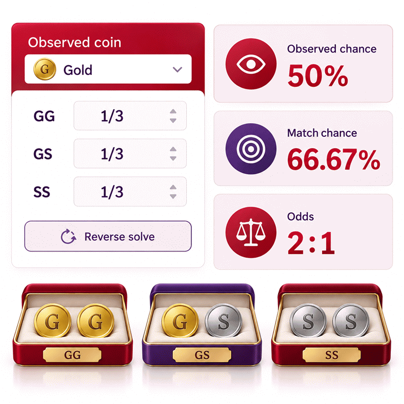
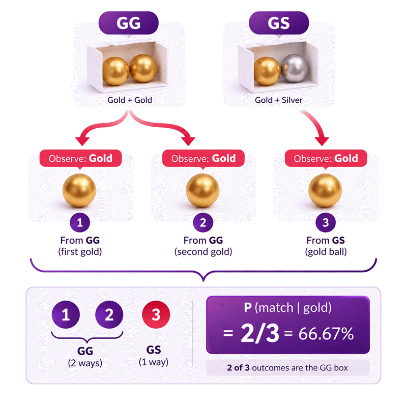
Bertrand’s Box Paradox Calculator shows why observing one gold coin changes the probability of the box you selected. In the classic setup, one box contains two gold coins, one contains gold and silver, and one contains two silver coins. After gold is observed, three gold-producing first-draw outcomes remain. Two come from the gold-gold box, while one comes from the mixed box. The hidden coin therefore matches gold with probability 2/3, or about 66.6667%.
- The classic matching probability is exactly 2/3.
- The tempting 1/2 answer incorrectly treats surviving boxes as equally likely.
- Bayesian updating gives posterior probabilities of 2/3 for GG and 1/3 for GS.
- Silver observations produce the symmetric result.
- Weighted box selection supports unequal prior probabilities.
- Reverse solving can calculate one missing box weight from a valid target result.
- Monte Carlo simulation approaches the analytical result as trials increase.
- Impossible and non-identifiable reverse states should be reported instead of forced.
The Bertrand’s Box Paradox Calculator on AxiCalculator combines exact probability, weighted scenarios, reverse solving, and simulation so users can test both the answer and the reasoning behind it.
Assumptions used in this calculator
- Each box-selection weight is treated as a non-negative relative probability weight.
- At least one box-selection weight must be greater than zero.
- A box is selected according to the entered relative weights.
- Each coin inside the selected box is equally likely to be drawn.
- Gold and silver observations are treated symmetrically by the probability model.
- Observed-color conditioning excludes outcomes inconsistent with the observed coin.
- The mixed box contains exactly one gold and one silver coin.
- Forward calculations use full precision before display rounding.
- Reverse solving requires exactly one box weight to be unknown.
- Some boundary probabilities cannot identify a unique missing weight.
- Simulation rounds are independent samples from the same probability model.
- Simulation estimates may differ slightly from exact analytical probabilities.
- Results assume unbiased coin selection within every selected box.
Results are rounded for display.
Internal calculations use full precision.
Formulas Used in Bertrand's Box Paradox Variables :
1. Total Selection Weight
2. Probability of Observing the Selected Color
The observed event is usable for conditioning only when 2s + m is greater than zero.
3. Conditional Matching Probability
This is the exact probability that the hidden coin matches the observed color.
4. Same-Color Weight from Matching Probability
A unique finite solution requires q below 1 and a compatible known mixed weight.
5. Mixed Weight from Matching Probability
A unique finite solution requires q above 0 and a compatible known same-color weight.
6. Same-Color Weight from Observed-Color Probability
The denominator requires p below 1, and the solved weight must be non-negative.
7. Mixed Weight from Observed-Color Probability
When p equals 0.5, this equation may become non-identifiable or incompatible.
8. Opposite-Color Weight from Observed-Color Probability
A unique finite solution requires p above 0 and a non-negative solved weight.
9. Simulated Observed-Color Probability
10. Simulated Conditional Matching Probability
This estimate is defined only when at least one qualifying observed-color round exists.
11. Matching Odds
At q = 0 the odds are 0 : 1, and at q = 1 they are 1 : 0.
s = homogeneous box weight matching the observed color.
m = mixed GS box weight.
o = homogeneous box weight opposite the observed color.
W = total box-selection weight.
p = exact probability of observing the selected color.
q = exact conditional probability that the hidden coin matches.
N = total simulation rounds.
NO = simulation rounds producing the requested observed color.
NM = qualifying rounds where the hidden coin also matches.
psim = simulated observed-color probability.
qsim = simulated conditional matching probability.
Variables & Definitions
View a complete list of all variables used in this calculator, including definitions and units
Bertrand's Box Paradox Variables and Probability Parameters
| Variable | Meaning | Type | Valid Domain | Role |
|---|---|---|---|---|
a |
GG box selection weight | Dimensionless weight | 0 to 1,000,000,000,000 | Controls the relative probability of selecting the two-gold box. |
b |
GS box selection weight | Dimensionless weight | 0 to 1,000,000,000,000 | Controls the relative probability of selecting the mixed box. |
c |
SS box selection weight | Dimensionless weight | 0 to 1,000,000,000,000 | Controls the relative probability of selecting the two-silver box. |
s |
Same-color homogeneous box weight | Dimensionless weight | 0 to 1,000,000,000,000 | Equals GG for Gold observation and SS for Silver observation. |
m |
Mixed-box weight | Dimensionless weight | 0 to 1,000,000,000,000 | Equals the GS box weight for either observed color. |
o |
Opposite-color homogeneous box weight | Dimensionless weight | 0 to 1,000,000,000,000 | Equals SS for Gold observation and GG for Silver observation. |
W |
Total selection weight | Dimensionless weight | Greater than 0 | Normalizes all box-selection weights. |
p |
Probability of observing the selected coin color | Probability | 0 to 1 | Measures how often the selected color appears on the first draw. |
q |
Conditional probability that the other coin matches | Probability | 0 to 1 | Primary exact result after conditioning on the observed color. |
N |
Total simulation rounds | Integer count | 100 to 200,000 | Controls Monte Carlo sample size. |
N_O |
Rounds matching the requested observed color | Integer count | 0 to N | Denominator for the simulated conditional probability. |
N_M |
Qualifying rounds where the other coin also matches | Integer count | 0 to N_O | Numerator for the simulated matching probability. |
p_sim |
Simulated observed-color probability | Estimated probability | 0 to 1 | Monte Carlo estimate of p. |
q_sim |
Simulated matching probability | Estimated probability | 0 to 1 | Monte Carlo estimate of q. |
Unit Conversion Table
Probability Representation and Relative Weight Conversion Table
| Unit Group | Unit Name | Symbol | Equivalent in Decimal Probability | Used For |
|---|---|---|---|---|
| Probability Representation | Decimal Probability | p | p | Internal probability calculations, Bayesian updates, and reverse solving |
| Probability Representation | Percentage | % | x% = x / 100 | User-facing probability inputs, exact results, and simulation results |
| Probability Representation | Odds Ratio | r : 1 | p = r / (1 + r) | Displaying matching odds relative to the non-matching outcome |
| Dimensionless Selection Scale | Relative Box Weight | w | w / (a + b + c) | Converting GG, GS, or SS relative weights into box-selection probabilities |
Example Calculation
Observed coin: Gold
GG weight = 3, GS weight = 2, SS weight = 5
The larger GG weight makes a matching Gold outcome more likely after Gold is observed.
The SS box affects the overall chance of observing Gold but not the conditional match chance.
After Gold is observed, only the GG and GS boxes remain possible.
The resulting 75% matching probability corresponds to matching odds of 3 : 1.
Observed coin: Gold
GS weight = 2
SS weight = 5
GG weight = unknown
Required matching probability = 75%
A 75% matching target requires the GG weight to be three when the GS weight is two.
The SS weight does not affect this specific conditional matching equation.
Using GG = 3 and GS = 2 reproduces a 75% exact matching probability.
With SS = 5, the overall probability of observing Gold is 40%.
Results are rounded for display.
Internal calculations use full precision.
Calculations Disclaimer
Why Does Bertrand’s Box Paradox Give 2/3 Instead of 1/2?
A real problem appears the moment someone says, “Two boxes are left, so the odds are 50-50.” That shortcut feels reasonable. It is also the step that breaks the calculation. Bertrand’s Box Paradox is not decided by counting box labels. It is decided by counting how strongly each remaining box could have produced the coin you observed.
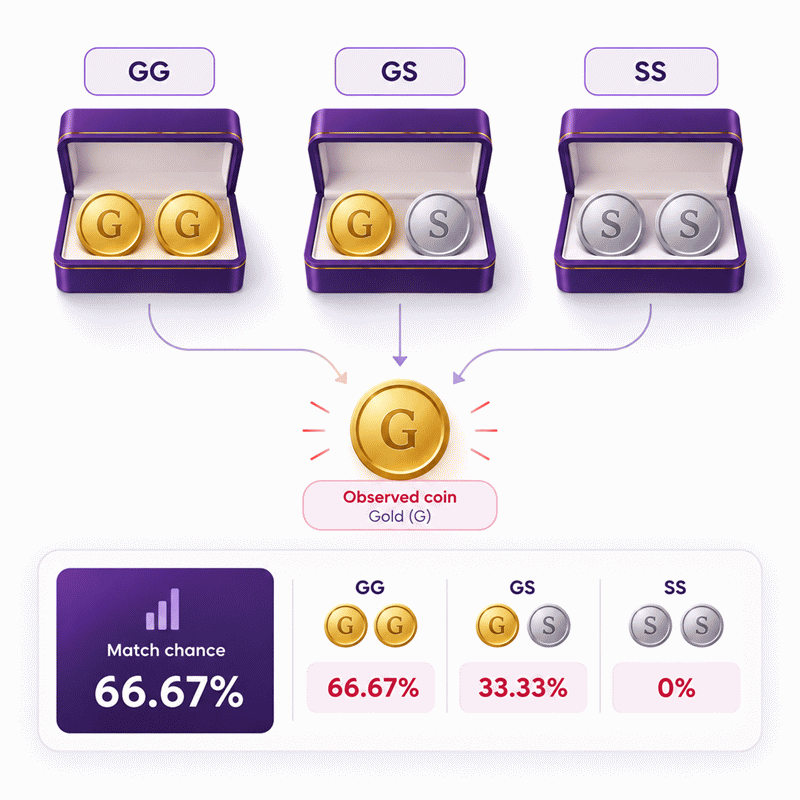
Start with three boxes. One contains two gold coins. One contains one gold and one silver coin. The third contains two silver coins. A box is selected. One coin is revealed. It is gold. The key question is now conditional: given that gold appeared, how likely is each box?
The gold-gold box can produce a gold observation in two ways. The mixed box can produce that observation in only one way. The silver-silver box cannot produce it at all. That creates three surviving gold-producing outcomes. Two point to the gold-gold box. One points to the mixed box.
The result follows immediately: two favorable outcomes out of three relevant outcomes. The hidden coin therefore matches gold with probability 2/3, or about 66.6667%.
QUICK MAP: 3 possible observed-gold coins → 2 belong to GG → 1 belongs to GS → match probability = 2/3.
What Changes the Moment a Gold Coin Is Observed?
The practical problem is that people often treat the observation as decoration. It is not. Seeing gold changes what you should believe about the selected box.
Before the draw, equal box selection gives every box the same starting chance. After gold appears, the silver-silver box is eliminated. More importantly, the two surviving boxes do not inherit equal probability. Their ability to generate gold differs.
The gold-gold box guarantees a gold first coin. The mixed box produces gold only half the time. Evidence that is twice as compatible with one hypothesis should not leave both hypotheses equally weighted.
This is why the puzzle matters beyond its coins. It trains a habit that is useful throughout statistics: ask how likely the evidence would be under each possible explanation.
Why Two Remaining Boxes Do Not Mean Equal Odds
A common real-world mistake is converting “two possibilities” into “two equally likely possibilities.” Those statements are not equivalent.
After gold appears, GG and GS remain possible. Yet GG had two routes to the observation. GS had one. The evidence therefore favors GG.
If you ignore those routes, you throw away information contained in the observation. That is exactly why 1/2 looks tempting. It counts names. The correct method counts probability mass.
A useful mental test is simple. Ask whether both surviving scenarios were equally capable of producing what you just saw. If not, equal posterior odds are usually unjustified.
The Three Gold-Producing Outcomes That Decide the Answer
Imagine labeling the three gold coins individually. Two labels sit inside GG. One sits inside GS. After a gold coin is observed, it must be one of those three labels.
If either GG gold coin was selected, the hidden coin is gold. If the GS gold coin was selected, the hidden coin is silver. That leaves two matching cases and one non-matching case.
This compact view removes nearly every source of confusion. It also provides a fast independent check for the classic result.
How Conditional Probability Rebuilds the Sample Space
The real problem in conditional probability is often not arithmetic. It is deciding which outcomes still matter after new information arrives.
Before a coin is observed, all six coin positions matter. After gold appears, the three silver first-draw positions no longer belong to the conditioned sample space. The calculation must therefore work with the surviving probability mass.
This is why Bertrand’s Box Paradox is such a useful statistics test. The numbers are simple, but the sample-space update must be correct.
Prior Probability Before Any Coin Is Seen
Before any coin is revealed, no evidence favors one classic box over another. Each box therefore begins with the same selection probability when selection is uniform.
That starting probability is called the prior. A prior describes the model before the new observation is included.
Equal priors are important in the classic puzzle. They are not a universal requirement. A generalized calculator can assign different relative selection weights to GG, GS, and SS. Once those priors change, the posterior result can change too.
Likelihood: How Strongly Each Box Predicts the Observation
A real analysis fails if it uses priors but ignores how each box produces the evidence. That second ingredient is the likelihood.
For a gold observation, GG has likelihood 1. GS has likelihood 1/2. SS has likelihood 0. These three numbers describe how compatible each box is with what happened.
The likelihood is why the observation contains information. Gold is not equally expected under every box. It favors the hypothesis that contains more gold-producing positions.
EVIDENCE LADDER: GG predicts gold perfectly → GS predicts gold half the time → SS cannot predict gold.
From Prior Weights to Posterior Box Probabilities
The practical task is to combine what was believed before the draw with how well each box predicts the observed coin.
Multiply each prior weight by its likelihood. Then compare only those surviving weighted paths. With equal classic priors, GG receives twice the surviving weight of GS. SS receives none.
Normalize those values and the posterior becomes 2/3 for GG, 1/3 for GS, and 0 for SS. The other coin matches gold exactly when the selected box is GG, so the matching probability is also 2/3.
How Bayes’ Rule Explains Bertrand’s Box Paradox
The practical difficulty with Bayes’ rule is that users often memorize symbols without seeing what they mean. In this puzzle, every term has a physical interpretation.
The prior says how likely a box was before the draw. The likelihood says how well that box predicts the observed color. The evidence measures the total chance of seeing that color. The posterior tells you how plausible the box is after seeing the color.
For the classic gold observation, the total probability of gold is 1/2. The joint contribution from choosing GG and then seeing gold is 1/3. Dividing 1/3 by 1/2 produces 2/3.
That is Bayes’ rule without mystery. It is simply a disciplined way to update probability after evidence arrives.
Why the Gold-Gold Box Receives Twice the Posterior Weight
A frequent problem is assuming the 2/3 result comes from a trick. It does not. GG receives twice the posterior weight because it offers twice as many gold-producing first-draw positions as GS.
Both gold coins in GG satisfy the observation. Only one coin in GS does. When the first coin is known to be gold, those paths determine the relative posterior weight.
This is also why the same reasoning works for a silver observation. SS then supplies two silver-producing positions. GS supplies one. The posterior reverses symmetrically.
What the Normalization Step Actually Does
A real calculation can produce correct relative weights but still fail to report valid probabilities. Normalization solves that problem.
After the observation, the surviving weights must be rescaled so their total equals one. In the classic gold case, the relative posterior weights are 2 for GG and 1 for GS. Their total is 3. Dividing by 3 produces 2/3 and 1/3.
Normalization does not create new evidence. It simply converts surviving probability mass into a valid posterior distribution.
Reading the Final 2:1 Posterior Odds
Some users understand odds more quickly than percentages. A probability of 2/3 corresponds to odds of 2:1 in favor of a match.
That means the matching outcome carries twice the conditional probability mass of the non-matching outcome. It does not mean a match is guaranteed. It means two matching paths exist for every one non-matching path in the classic conditioned sample space.
The odds view is useful because it exposes the central structure immediately: after gold is known, GG outweighs GS by two to one.
How a Weighted Bertrand Box Model Goes Beyond the Classic Puzzle
A real limitation appears when the boxes are not equally likely to be selected. The textbook answer no longer covers every case.
A weighted model solves that problem. Give GG, GS, and SS non-negative relative selection weights. Those weights represent prior selection propensity. They do not need physical units.
For a selected observed color, let the matching homogeneous box have weight s. Let the mixed box have weight m. Let the opposite homogeneous box have weight o.
The conditional matching probability depends on the gold- or silver-producing paths:
q = 2s / (2s + m)
The overall chance of observing the selected color is:
p = (2s + m) / [2(s + m + o)]
These relationships preserve the classic puzzle when all three original box weights equal one.
What Happens When GG, GS, and SS Are Not Equally Likely?
A practical analyst may know that some boxes are selected more often than others. Equal priors would then misrepresent the experiment.
Suppose GG has weight 3, GS has weight 2, and SS has weight 5. For a gold observation, GG contributes six gold-producing weight units. GS contributes two. The conditional match chance becomes 6/8, or 75%.
Notice what happened. The famous 2/3 result changed because the prior selection process changed. Conditional probability always belongs to a clearly defined sampling process.
Why Relative Weights Preserve the Probability Model
Users sometimes worry that weights must add to one. They do not. Relative weights can be normalized automatically.
Weights 1:1:1 and 10:10:10 describe the same prior proportions. Multiplying every weight by one positive constant changes their scale but not their ratios.
This makes relative weights practical. Users can enter counts, frequencies, or proportional selection weights without converting them manually into percentages first.
When the Opposite-Color Box Matters and When It Does Not
A subtle problem appears when users expect every box weight to affect every output. That is not true.
After gold is observed, the SS box cannot be the selected box. Therefore, its weight does not affect the conditional probability that the hidden coin matches gold. That result depends on GG and GS.
However, SS still affects the overall chance of observing gold before conditioning. Increasing SS makes a gold first draw less common across the full experiment.
This distinction is useful when checking calculations. One output can be insensitive to a parameter that still influences another output.
Can Bertrand’s Box Paradox Be Solved Backward?
A real project does not always begin with every box weight known. Sometimes the desired probability is known and one input is missing.
That is where reverse solving becomes useful. Instead of asking, “What probability follows from these weights?” the user can ask, “What missing weight would create this target probability?”
This turns the tool from a one-direction example into a compact inverse-probability model.
Finding a Missing Same-Color Box Weight from a Target Probability
Suppose gold is observed. The GS weight is 2. The desired matching probability is 75%. The GG weight is unknown.
Using the conditional relationship, the required same-color weight is 3. A forward check confirms the result:
2 × 3 / (2 × 3 + 2) = 6/8 = 0.75.
That verification step matters. Every reverse result should reproduce the target when inserted back into the forward model.
Finding the Mixed-Box Weight from a Desired Match Chance
Another real problem starts with the same-color weight known but the mixed weight unknown.
If the same-color weight is fixed, increasing the mixed-box weight reduces the conditional match chance. The mixed box creates observed-color outcomes whose hidden partner is the opposite color.
This relationship lets the calculator solve the required mixed weight from a chosen target probability. It also gives users a direct way to study sensitivity.
When Reverse Solving Has No Unique Finite Answer
A reverse calculator becomes dangerous if it always forces a number. Some target values do not identify one finite missing weight.
A boundary probability may require an infinite limit. Another configuration may allow many different missing values to produce the same result. Some combinations imply a negative weight, which is invalid for this model.
AxiCalculator should reject those cases clearly. “No unique finite solution” is a better result than a misleading number.
REVERSE CHECK: solve the missing weight → insert it into the forward equation → confirm the target → reject impossible or non-unique states.
Does Monte Carlo Simulation Really Converge to Two Thirds?
A real simulation can worry users because it rarely lands on exactly 66.6667%. That is expected.
The analytical probability describes the model exactly. A Monte Carlo run describes one random sample from that model. With 100 trials, the result can wander noticeably. With thousands of trials, it usually settles closer to the analytical probability.
The key is to simulate the correct experiment. Select a box according to its prior weights. Select one of its two coins fairly. Keep only trials where the first coin matches the requested observed color. Then check the hidden coin.
The conditional simulation estimate uses matching qualifying trials divided by all qualifying observed-color trials.
Why Small Simulations Wander Around the Exact Result
A common user concern is seeing a simulated result such as 64% or 69% when the exact answer is 66.6667%.
Random sampling naturally creates variation. A short run can contain more GG observations or more GS observations than their long-run proportions suggest. Nothing has gone wrong simply because the estimate is not exact.
As the sample grows, large deviations become less typical. The estimate usually moves closer to the theoretical value.
How to Read Qualifying Trials Correctly
A simulation produces a serious error if it divides by every trial instead of the conditioned trials.
If the question begins “given that gold was observed,” only trials with an observed gold coin belong in the denominator. Silver-first trials are not failures. They are outside the conditioned sample.
Among those qualifying gold trials, count how many have a gold hidden coin. That ratio estimates the required conditional probability.
Exact Probability and Simulated Probability Serve Different Jobs
A practical workflow should not force users to choose between mathematics and simulation. They answer different needs.
The exact calculation gives the model’s true probability. Simulation shows how random data generated by that model behaves. Reverse solving reveals which inputs can produce a target result.
Used together, these three views turn a famous puzzle into a useful probability laboratory. You can change priors, switch the observed color, test edge cases, and see how evidence reshapes the posterior.
Use AxiCalculator when you want the answer immediately, then change the setup until the reason behind that answer becomes intuitive. The most useful lesson is not memorizing 2/3. It is learning to ask how strongly each possible explanation predicts the evidence you actually observed.
Frequently Asked Questions
Why does seeing one gold coin make the gold-gold box more likely?
Does the answer stay 2/3 if the boxes are selected with different probabilities?
Why does a Monte Carlo result not always display exactly 66.6667%?
What changes if the first observed coin is silver instead of gold?
Why can a reverse Bertrand box calculation have no unique solution?
How should an engineer or analyst validate a generalized weighted result?
Why can the opposite-color box affect one output but not the matching probability?
Our engineers are here to help you get it right.