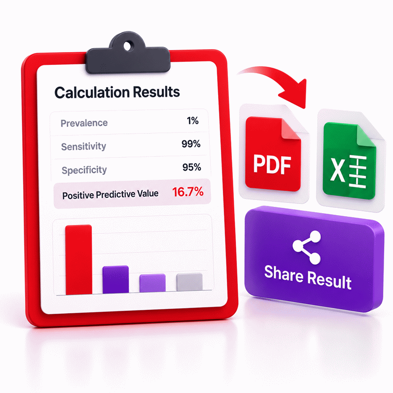
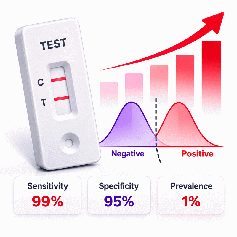
False Positive Paradox Calculator
- Last formula update:

Decimal & Rounding Policy
- All calculations use full internal precision without rounding intermediate values.
- Displayed results use up to 10 decimal places and remove unnecessary trailing zeros.
- Reverse-solved inputs retain up to 12 significant digits before display.
- Percentage and decimal units remain mathematically equivalent during every calculation.
- Display rounding never changes the underlying probability used by the calculator.
Valid range
- Base rate must be greater than 0% and strictly less than 100%.
- Sensitivity must be greater than 0% and no more than 100%.
- Specificity must be greater than 0% and no more than 100%.
- Positive predictive value must be greater than 0% and no more than 100%.
- Decimal probability inputs use equivalent ranges between 0 and 1.
- Exactly one parameter may remain unknown when using reverse calculation.
- Negative, zero where prohibited, non-finite, or out-of-range values are invalid.

Wylena Brantford
Reviewers:
Valdren Clyforde
Zenara Dentwick
Check our editorial policy
September 17, 2026
1.0.0
Initial calculator and formula release.
Our engineers are here to help you get it right.
What Does the False Positive Paradox Calculator Tell You About a Positive Result?
False Positive Paradox Calculator shows why a positive result can be less reliable than an impressive accuracy percentage suggests. The result depends on how common the target condition is, how well the test detects true cases, and how effectively it rejects negative cases.
- Low prevalence can create more false positives than true positives.
- Sensitivity describes detection of real positive cases.
- Specificity describes correct rejection of real negative cases.
- Positive predictive value measures how many positive results are actually correct.
- A large negative population can magnify a small false-positive rate.
- Expected counts make the statistical imbalance easier to understand.
- The same effect appears in screening, fraud detection, cybersecurity, and machine learning.
- Population choice can change predictive value without changing test performance.
The False Positive Paradox Calculator helps you interpret a positive signal within its real statistical context. Use the result to compare true and false positives, understand how prevalence changes reliability, and avoid confusing sensitivity with the probability that a positive result is correct.
Assumptions used in this calculator
- Base rate represents condition prevalence in the tested population.
- Sensitivity and specificity are treated as fixed test characteristics.
- Input probabilities use consistent percentage or decimal representations.
- Base rate remains strictly between zero and one.
- Sensitivity, specificity, and PPV must exceed zero.
- Sensitivity, specificity, and PPV cannot exceed one.
- Exactly one unknown may be reverse-solved at a time.
- The tested population is sufficiently large for expected-count interpretation.
- Counts per 1,000 are statistical expectations, not observed outcomes.
- Test outcomes are assumed independent across tested individuals.
- Test characteristics are assumed applicable to the selected population.
- Intermediate calculations retain full numerical precision.
- Displayed rounding does not change the underlying calculated probability.
Results are rounded for display.
Internal calculations use full precision.
Formulas Used in False Positive Paradox Calculator :
Positive Predictive Value
Reverse Solve for Base Rate
Reverse Solve for Sensitivity
Reverse Solve for Specificity
False Discovery Rate
False Positive Rate
Expected True Positives per 1,000
Expected False Positives per 1,000
False Positives to True Positives Ratio
- BR = base rate or prevalence.
- SE = sensitivity.
- SP = specificity.
- PPV = positive predictive value.
- FDR = false discovery rate.
- FPR = false positive rate.
- TP1000 = expected true positives per 1,000 tested individuals.
- FP1000 = expected false positives per 1,000 tested individuals.
- R = false positives to true positives ratio.
Variables & Definitions
View a complete list of all variables used in this calculator, including definitions and units
False Positive Paradox Calculator Variables and Statistical Parameters
| Variable | Meaning | Unit | Valid Range | Used For |
|---|---|---|---|---|
| BR | Base rate or prevalence of the condition | % or decimal | 0 < BR < 1 | Prior probability of the condition |
| SE | Sensitivity of the test | % or decimal | 0 < SE ≤ 1 | Probability of a positive result when the condition is present |
| SP | Specificity of the test | % or decimal | 0 < SP ≤ 1 | Probability of a negative result when the condition is absent |
| PPV | Positive predictive value | % or decimal | 0 < PPV ≤ 1 | Probability that a positive result is a true positive |
| FDR | False discovery rate | % or decimal | 0 ≤ FDR < 1 | Proportion of positive results expected to be false positives |
| FPR | False positive rate | % or decimal | 0 ≤ FPR < 1 | Probability of a positive result when the condition is absent |
| TP1000 | Expected true positives per 1,000 tested individuals | people per 1,000 | 0 to 1,000 | Expected true-positive count |
| FP1000 | Expected false positives per 1,000 tested individuals | people per 1,000 | 0 to 1,000 | Expected false-positive count |
| R | False positives to true positives ratio | ratio | R ≥ 0 | Compares expected false positives with true positives |
Unit Conversion Table
Percentage to Decimal Probability Conversion
| Unit Group | Unit Name | Symbol | Equivalent in Decimal | Used For |
|---|---|---|---|---|
| Popular Units | Percent | % | 1% = 0.01 | BR, SE, SP, PPV, FDR, and FPR |
Decimal to Percentage Probability Conversion
| Unit Group | Unit Name | Symbol | Equivalent in Percent | Used For |
|---|---|---|---|---|
| Scientific Units | Decimal Probability | decimal | 0.01 = 1% | BR, SE, SP, PPV, FDR, and FPR |
Example Calculation
The condition occurs in only 2.5% of the tested population.
High specificity limits the number of false positive results.
A positive result has an estimated 62.13592233% probability of being correct.
About 14.625 false positives are expected for every 1,000 tested individuals.
The reverse calculation solves the missing base rate from three known probabilities.
The resulting prevalence is approximately 2.127659574% of the tested population.
False positives exceed true positives because the positive predictive value is 40%.
The model therefore expects approximately 1.5 false positives per true positive.
Results are rounded for display.
Internal calculations use full precision.
Calculations Disclaimer
Why Can a Positive Result Be Less Reliable Than It Sounds?
A positive result can create immediate confidence. That confidence may be statistically misplaced. The False Positive Paradox Calculator exposes that hidden problem. The False Positive Paradox Calculator shows why accuracy alone cannot answer the real question.
Imagine a screening system that rarely makes mistakes. The number sounds reassuring. Yet the event being detected may be extremely rare. Most tested people therefore belong to the negative group. Even a small error rate can affect many people.
This creates an important imbalance. True positives come from a small group. False positives come from a much larger group. The larger group can dominate the final positive results.
The result feels strange because human intuition focuses on test performance. It often ignores how common the target condition was beforehand. That missing context changes everything.
A positive result answers only part of the decision problem. You also need to know the population behind that result. A reliable interpretation considers prevalence, sensitivity, specificity, and predictive value together.
This issue matters whenever rare events are being detected. Medical screening is only one application. Fraud systems face the same structure. Security alerts face it too. Spam filters and moderation systems can also experience it.
The calculator helps separate two questions. First, how well does the test detect real cases? Second, how believable is a positive result in this population?
Those questions sound similar. They are not interchangeable. Confusing them is the central reason this paradox surprises people.
The safest interpretation starts with context. Ask how common the event is. Then inspect the test characteristics. Finally, evaluate the positive result itself.
This order prevents a familiar mistake. It stops one impressive percentage from dominating the entire decision.
When Low Prevalence Changes the Meaning of Test Accuracy
A rare condition creates a difficult screening environment. Almost everyone tested belongs to the negative group. That fact can outweigh excellent test performance.
Suppose the target event becomes less common. The pool producing true positives shrinks. The negative pool becomes relatively larger. False positives can therefore occupy more positive results.
The test did not suddenly become worse. Its sensitivity may remain unchanged. Its specificity may also remain unchanged. The surrounding population changed the meaning of its output.
This distinction is essential for responsible interpretation. Predictive value belongs to a test-population combination. It is not simply a permanent label attached to a test.
A result measured in one setting may not transfer cleanly elsewhere. A specialist clinic can contain many high-risk cases. A general screening population may contain very few. Identical test characteristics can therefore produce very different positive-result reliability.
This is why population selection deserves attention. Using an unrelated prevalence estimate can create false confidence. It can also create unnecessary alarm.
The chain above captures the practical mechanism. The problem begins before the test result appears. It begins with the size of each underlying group.
This insight also explains targeted screening. A carefully selected population may have a higher prior probability. A positive result can then carry more information.
Targeting does not magically improve the test itself. It changes the context in which the test operates.
That distinction matters for analysts, clinicians, engineers, and data scientists. It prevents them from treating one performance number as universally meaningful.
The Hidden Competition Between True Positives and False Positives
A dashboard can show an impressive accuracy figure. That figure may hide the comparison that matters most. Positive results contain two competing groups.
One group contains correct positive detections. The other contains incorrect positive detections. The useful question is how those groups compare.
When correct positives dominate, a positive signal has stronger predictive meaning. When incorrect positives dominate, caution becomes more important.
This is easier to understand with expected counts. Think about a fixed group of tested people. Some truly have the target condition. Others do not.
Sensitivity controls how many real cases are detected. Specificity controls how many non-cases are correctly rejected. The remaining errors shape the false-positive burden.
Low prevalence makes this burden particularly important. There may be thousands of negatives for every true case. A tiny error applied thousands of times can become a large number.
This perspective reduces cognitive bias. Instead of asking whether a test sounds accurate, ask what creates the positive pool.
The same reasoning works for automated systems. A fraud detector may inspect millions of normal transactions. A security system may scan millions of harmless events. An AI moderator may inspect mostly legitimate content.
Each system can generate many false alerts without being obviously defective. Rare-event detection simply demands stricter interpretation.
Why Does Base Rate Matter More Than Most People Expect?
A user receives an alert and focuses on the alert. The earlier probability disappears from attention. That is exactly where bad interpretation starts.
The base rate describes how common the target event is before new evidence appears. It gives the result its starting context.
A positive signal updates that starting point. It does not erase it. Strong evidence can move probability substantially. Yet an extremely low starting probability can still matter.
This is why the same positive signal can mean different things. A high-risk population begins from one position. A low-risk population begins from another.
Ignoring this difference produces base-rate neglect. The result often feels intuitive at first. It can be statistically wrong.
People naturally notice vivid new evidence. A positive test feels concrete. A background prevalence statistic feels abstract. The brain therefore gives the positive result more attention.
A good calculator counters that tendency. It forces the starting probability back into the decision.
How Prior Probability Shapes the Meaning of New Evidence
A screening result does not exist in isolation. Every interpretation begins with information available before testing.
For this calculator, prevalence provides that starting information. It represents the proportion expected to have the condition within the selected population.
Changing that population can change the result dramatically. The test itself may remain identical.
This explains why broad population screening differs from targeted evaluation. A broad population can contain very few true cases. A targeted population may contain many more.
The positive result therefore carries different practical weight. This is not a contradiction. It is normal conditional probability.
Analysts should always ask where the prevalence value came from. It should represent the population actually being evaluated.
A national average may be inappropriate for a specialized subgroup. A high-risk clinic estimate may be inappropriate for general screening.
Choosing the wrong base rate can shift the final interpretation. That error can be larger than ordinary display differences.
How Do Sensitivity and Specificity Affect a Positive Result?
A team may celebrate high sensitivity while false alerts keep growing. The missing issue may be specificity.
Sensitivity measures how effectively real positive cases are detected. It protects against missed positive cases.
Specificity works on the opposite population. It measures how effectively real negatives are rejected.
Both matter. Their practical influence changes with the population.
In rare-event screening, the negative population can be enormous. Specificity therefore becomes especially important. A small loss in specificity can create many false positives.
Increasing sensitivity cannot always fix that problem. Better detection of scarce true cases may add relatively few positives. Meanwhile, false positives continue arriving from the huge negative group.
This is why test evaluation needs more than one headline metric. Sensitivity alone cannot describe positive-result reliability. Specificity alone cannot either.
Their interaction with prevalence determines what users actually experience after a positive result.
Why Specificity Becomes Critical in Low-Prevalence Populations
A rare-event detector processes mostly negative cases. That makes every specificity error more visible at scale.
Consider the operational problem rather than the percentage. Every false alert can require review. Reviews consume time, money, attention, and sometimes emotional energy.
A system producing thousands of false alerts may still report attractive sensitivity. The operational burden remains real.
For screening systems, reducing false alarms can therefore be as important as finding more positives. The balance depends on consequences.
A missed dangerous case can be costly. A false alarm can also be costly. Different applications assign different costs to each error.
The calculator does not choose those costs for you. It shows the statistical balance behind the positive results.
That balance helps users ask better questions. Is the positive pool mostly correct? Are false alerts dominating? Is the selected population appropriate?
What Does Positive Predictive Value Tell You After a Positive Result?
A positive result arrives, but the user wants a different answer. The user wants to know whether the positive is likely correct.
Positive predictive value addresses that practical question. It describes the share of positive results expected to represent true positive cases.
This makes PPV highly intuitive once its meaning is clear. A larger value means positive signals contain a larger proportion of true positives.
A lower value means false positives occupy more of the positive-result pool.
PPV should not be confused with sensitivity. Sensitivity begins with people who truly have the condition. PPV begins with people who received positive results.
The direction of conditioning changes the question. That small wording change creates a major statistical difference.
This distinction is useful beyond diagnostics. Machine-learning practitioners know a related concept as precision. Alerting systems face the same question: how many generated alerts are actually correct?
Understanding this connection makes the calculator useful across several fields.
Why PPV Answers a Different Question Than Sensitivity
A manager sees 99% sensitivity and assumes almost every alert is correct. That conclusion does not follow.
Sensitivity evaluates known positive cases. It asks how many were successfully detected.
PPV evaluates generated positive results. It asks how many of those positives are correct.
Those populations are different. Their denominators are different. Their practical meanings are different.
The confusion becomes dangerous with rare events. High sensitivity can coexist with modest PPV. The system finds most real cases but still generates many false alerts.
Users should therefore read results in the correct order. First understand the population. Then understand the test behavior. Finally interpret the positive result.
This sequence is slower than trusting one accuracy number. It is also much safer.
Where Does the False Positive Paradox Appear Outside Medicine?
A fraud team may investigate hundreds of alerts and find few real fraud cases. The same mathematics can explain why.
Fraud is usually rare relative to legitimate activity. A detector processes a massive normal population. Even a small false-positive rate can create a large review queue.
Cybersecurity systems face a similar challenge. Genuine attacks are uncommon compared with normal events. Poor alert precision can overwhelm analysts.
Spam filters also operate on class imbalance. Moderation systems encounter it when prohibited content is rare. Manufacturing inspection systems can experience it with rare defects.
Airport screening provides another intuitive case. Serious threats are extremely uncommon. A detector must operate within that tiny base rate.
These examples reveal the broader lesson. The paradox is not about medicine. It is about rare-event detection.
Any binary classifier can face the same structure. The labels change, but the statistical problem remains.
Fraud Detection, Cybersecurity, Spam Filters, and Rare Alerts
An operations team may think more alerts mean better protection. More alerts can also mean more noise.
Useful alert systems must balance detection and review burden. Excessive false positives consume scarce human attention.
This creates alert fatigue. Analysts may respond more slowly. Important alerts can disappear inside routine noise.
Understanding predictive value helps teams evaluate this risk. A system should not be judged only by detection rate.
The environment matters too. A model deployed on a different population can behave differently. The prevalence of target events may change.
This explains why performance should be monitored after deployment. Validation conditions are not permanent.
Why Machine Learning Models Can Fail on Rare Classes
A model can report impressive overall accuracy while barely identifying a rare class. Class imbalance creates that trap.
If almost every observation belongs to one class, predicting that class often looks accurate. The headline metric hides the failure.
Precision and recall provide more useful context. The same idea applies to false-positive analysis.
Rare-class systems need evaluation that respects the underlying distribution. Confusion-matrix counts help expose what a percentage can hide.
The key question is operational. What happens when this model processes the real population?
AxiCalculator helps translate that population structure into understandable positive-result reliability.
How Should You Interpret a False Positive Paradox Calculator Result?
A user sees several outputs and may focus on the largest number. Start with the result matching your question.
If the question concerns a positive signal, positive predictive value deserves immediate attention. It directly describes how much of the positive pool is expected to be correct.
Next, compare expected true positives with expected false positives. That comparison turns probability into an intuitive balance.
A false-positive-to-true-positive ratio above one deserves attention. It means false positive outcomes are expected to exceed true positives.
Then return to the inputs. Check whether the selected population is appropriate. Check whether the test characteristics represent the actual system.
A mathematically correct calculation can still be poorly interpreted when inputs lack context.
Which Result Deserves Your Attention First?
A positive test creates one practical question: how much should this positive result change confidence?
Start with predictive value. Then inspect the false-discovery share and expected counts.
Counts are especially useful for communication. Stakeholders often understand twenty alerts better than a small probability.
Do not treat the calculator as a verdict. Treat it as a probability interpreter.
The output describes what the supplied statistical model implies. Decisions still require domain context.
How Can Better Decisions Reduce the Impact of False Positives?
A screening program may generate too many false alarms. Changing interpretation alone will not fix operations.
Better population targeting can help. Improving specificity can help. Independent follow-up evidence may also improve confidence.
The best strategy depends on consequences. Some systems tolerate many false alerts to avoid missed cases. Others cannot afford that burden.
The important step is seeing the trade-off clearly.
AxiCalculator turns that trade-off into visible numbers. Users can change the inputs and observe how the result responds.
That interaction builds intuition faster than memorizing terminology. It also exposes assumptions hidden behind impressive accuracy claims.
Use the calculator to challenge intuition before making conclusions. Compare populations. Test alternative performance levels. Examine whether false positives dominate.
One positive result can feel definitive. Probability is usually more nuanced.
That nuance is precisely why the false positive paradox matters.
Frequently Asked Questions
Can a positive result be unreliable even when the test looks highly accurate?
Does the number of people tested change positive predictive value?
Why is a false-positive rate different from a false discovery rate?
Can this calculator be useful outside medical screening?
Why can specificity matter more than expected in a rare-event detection project?
What should an engineer check before using a calculated PPV in another population?
How can reverse solving help when designing a screening or alert system?
Our engineers are here to help you get it right.