Joint Probability Variables and Calculation
- Last formula update:

Decimal & Rounding Policy
- Probabilities are calculated internally as decimal values from 0 to 1.
- Intermediate calculations retain full available precision without manual rounding.
- Displayed results use up to 12 significant digits for readable output.
- Unit conversion occurs before display formatting to preserve the underlying probability.
- Reverse calculations use unrounded values to minimize cumulative rounding error.
- Exact boundary probabilities such as 0 and 1 remain unchanged.
Valid range
- P(A) must be between 0 and 1 inclusive.
- P(B) must be between 0 and 1 inclusive.
- P(A|B) must be between 0 and 1 when the condition is defined.
- P(A and B) must be between 0 and 1 inclusive.
- Percentage probability values must stay between 0% and 100%.
- Reverse conditional calculations require a positive divisor to produce a unique result.
- For independent events, joint probability cannot exceed either individual probability.
- For the dependent model, P(A and B) cannot exceed P(B).
- Values producing a probability below 0 or above 1 are invalid.

Wylena Brantford
Reviewers:
Valdren Clyforde
Zenara Dentwick
Check our editorial policy
September 16, 2026
1.0.0
Initial calculator and formula release.
Our engineers are here to help you get it right.
How Does a Joint Probability Calculator Find the Chance That Two Events Both Occur?
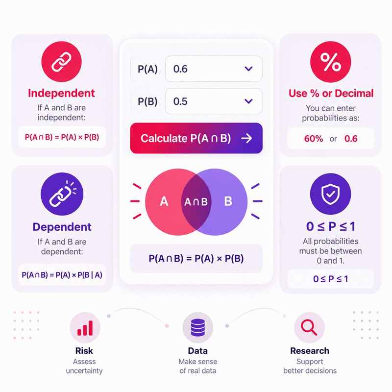
Joint Probability Calculator results depend first on the relationship between your events. Independent events use P(A∩B) = P(A) × P(B), because one event does not change the probability of the other. Dependent events require a conditional probability, such as P(A∩B) = P(A|B) × P(B).
- Use independent mode only when the events do not influence each other.
- Use dependent mode when one probability changes after another event occurs.
- P(A∩B) means that both specified events occur.
- Any valid probability must remain between 0 and 1.
- The joint probability cannot exceed either event required for the intersection.
- Reverse solving can recover a missing probability from two known values.
- A zero divisor can make reverse solving undefined rather than zero.
- Percentages and decimals represent the same probability on different scales.
The Joint Probability Calculator from AxiCalculator is most useful when you treat the relationship assumption as part of the calculation. Define the events first, choose the correct mode, enter the known values, then check whether the result makes logical sense.
Assumptions used in this calculator
- Each entered value represents a valid probability for the stated event.
- Users correctly identify whether the analyzed events are independent or dependent.
- Independent events do not change each other’s probability of occurring.
- Dependent calculations use P(A|B) as the required conditional probability.
- All probabilities refer to the same defined experiment or population.
- Probability values remain between zero and one after unit conversion.
- Percentage values represent probabilities, not percentage changes or percentage points.
- Input data is assumed accurate before calculations are performed.
- Reverse solving assumes the known values define a unique solution.
- Division by zero does not produce a valid reverse probability.
- Intermediate calculations retain full available numerical precision.
- Displayed rounding does not alter the internal calculated probability.
- Theoretical probabilities may differ from frequencies observed in finite samples.
Results are rounded for display.
Internal calculations use full precision.
Formulas Used in Joint Probability Variables and Calculation :
Probability Unit Normalization
- v
- Displayed probability value entered by the user.
- fu
- Conversion factor for the selected probability unit.
- p
- Normalized decimal probability used internally.
- Decimal: fu = 1
- Percent: fu = 0.01
- Per mille: fu = 0.001
- Basis point: fu = 0.0001
- Parts per million: fu = 0.000001
Independent Joint Probability
- P(A)
- Probability that event A occurs.
- P(B)
- Probability that event B occurs.
- P(A∩B)
- Probability that both independent events occur.
Dependent Joint Probability
- P(A|B)
- Probability that event A occurs given that event B occurs.
Variables & Definitions
View a complete list of all variables used in this calculator, including definitions and units
Joint Probability Variables and Calculation Parameters
| Variable | Meaning | Calculation Role | Valid Base Range | Common Display Units |
|---|---|---|---|---|
| v | User-entered or displayed probability value | Converted into the normalized decimal probability | Depends on the selected unit | Decimal, %, ‰, bp, ppm |
| fu | Conversion factor for the selected probability unit | Converts the displayed value into decimal probability | Positive conversion factor | 1, 0.01, 0.001, 0.0001, 0.000001 |
| p | Normalized decimal probability | Base value used for all calculations | 0 to 1 | Decimal |
| P(A) | Probability of event A | Independent-event input | 0 to 1 | Decimal, %, ‰, bp, ppm |
| P(B) | Probability of event B | Input in both relationship modes | 0 to 1 | Decimal, %, ‰, bp, ppm |
| P(A|B) | Probability of event A given event B | Dependent-event conditional input | 0 to 1 when defined | Decimal, %, ‰, bp, ppm |
| P(A∩B) | Probability that events A and B occur together | Joint probability result or reverse-solving input | 0 to 1 | Decimal, %, ‰, bp, ppm |
Unit Conversion Table
Joint Probability Unit Conversion Table
| Unit Group | Unit Name | Symbol | Equivalent in Decimal Probability | Used For |
|---|---|---|---|---|
| Popular Units | Percent | % | 1% = 0.01 | Common probability input and result display |
| Popular Units | Decimal Probability | 1 | 1 = 1 | Base calculations and normalized probability values |
| Scientific Units | Per Mille | ‰ | 1‰ = 0.001 | Probabilities and rates expressed per thousand |
| Scientific Units | Basis Point | bp | 1 bp = 0.0001 | Fine probability and rate differences |
| Scientific Units | Parts Per Million | ppm | 1 ppm = 0.000001 | Very small probabilities and rare-event rates |
Example Calculation
Suppose event A has a 72% probability and event B has a 45% probability.
Because the events are independent, their decimal probabilities are multiplied.
The calculated joint probability is 0.324, which equals 32.4%.
This means both events are expected to occur together with a 32.4% probability.
The joint probability is known as 21%, while P(B) is known as 35%.
The dependent-event formula is rearranged to solve the missing conditional probability.
Dividing 0.21 by 0.35 gives a decimal probability of 0.60.
The missing conditional probability P(A|B) is therefore 60%.
Results are rounded for display.
Internal calculations use full precision.
Calculations Disclaimer
How Can a Joint Probability Calculator Prevent the Most Common Probability Mistake?
A probability problem can look simple and still produce a wrong answer. The usual problem is not multiplication. It is choosing the wrong relationship between events. A Joint Probability Calculator helps by forcing that decision first. You decide whether the events are independent or dependent. The calculator then uses the matching probability relationship.
Joint probability answers one specific question. What is the chance that event A and event B both occur? The result is written as P(A∩B) or P(A and B). That distinction matters because the word “and” is doing real mathematical work.
Consider two unrelated events. Event A has a 60% probability. Event B has a 40% probability. If the events are independent, their joint probability is 24%. The result comes from multiplying 0.60 by 0.40.
Now change the situation. Suppose event B changes the chance of event A. The original 60% value may no longer apply after B occurs. A conditional probability is now needed. Using the independent formula would create a confident-looking but misleading result.
AxiCalculator keeps this choice visible. That helps you focus on the assumption before the arithmetic. It also supports reverse solving. You can enter the joint probability and one known factor. The remaining probability can then be calculated automatically.
This is useful for students, analysts, researchers, engineers, and decision makers. The calculation is short. The interpretation deserves more care.
When Should You Treat Two Events as Independent?
A common real problem starts with two percentages from different sources. It is tempting to multiply them immediately. That shortcut only works when one event does not change the probability of the other.
Suppose a fair coin is tossed. At the same time, a fair die is rolled. The coin result does not influence the die result. These events can be modeled as independent.
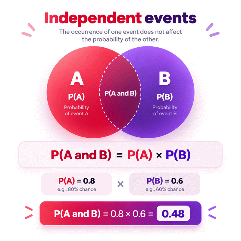
If event A has probability P(A), and event B has probability P(B), independence gives:
P(A∩B) = P(A) × P(B)
Imagine that P(A) is 0.75 and P(B) is 0.40. Their joint probability is 0.30. This means both specified events have a 30% chance of occurring together.
Why Independence Changes the Multiplication Rule
Independence means new information about one event does not change the other event’s probability. If B occurs, the probability of A stays P(A). In notation, P(A|B) equals P(A).
This is why the general multiplication rule becomes simple. The conditional factor can be replaced by the ordinary probability.
There is also a quick sense check. For independent events, the joint probability cannot exceed either factor. Both probabilities lie between zero and one. Multiplying them cannot make the result larger.
If your calculated joint probability exceeds one of the individual probabilities, inspect the inputs. A unit mistake or incorrect relationship may be present.
How to Test Whether One Event Changes the Other
Ask one practical question: after learning that B occurred, would you revise the chance of A?
If the answer is no, independence may be reasonable. If the answer is yes, the events should not be treated as independent.
Think about drawing cards. Drawing the first card without replacement changes the deck. The probability for the second draw therefore changes. With replacement, the original deck composition is restored. The draws can then follow an independent model.
This simple test often prevents a larger error than any rounding issue.
What Changes When the Events Are Dependent?
Dependent events create a different problem. The probability of one event depends on information about another. A marginal probability alone is no longer enough.
The general calculation can be written as:
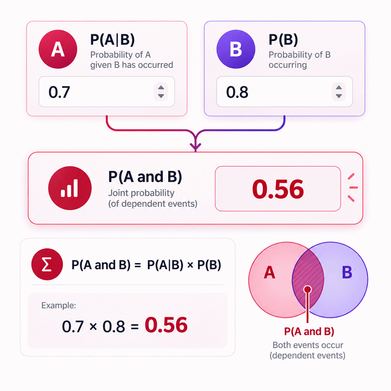
P(A∩B) = P(A|B) × P(B)
Here, P(A|B) means the probability of A after B is known to have occurred.
Suppose P(B) is 0.50. After B occurs, the probability of A becomes 0.70. The joint probability is therefore 0.35.
Notice what changed. We did not multiply the original unconditional probability of A by P(B). We used the probability that applies inside the condition created by B.
Why Conditional Probability Becomes the Critical Input
The word “given” changes the sample space. You are no longer asking about A across every possible case. You are asking about A only within cases where B occurred.
This distinction appears in reliability analysis, quality control, medical studies, finance, machine learning, surveys, and experimental work. A previous result can change the likelihood of the next event.
That does not mean dependence always increases risk. It may increase or decrease the conditional probability. The direction depends on the situation.
Choosing Between P(A|B) and P(B|A)
Conditional probability has direction. P(A|B) and P(B|A) usually mean different things.
You can calculate the same joint event using either consistent orientation:
P(A∩B) = P(A|B) × P(B)
or
P(A∩B) = P(B|A) × P(A)
The important rule is consistency. Do not combine a conditional probability with the wrong marginal factor.
This is especially important when labels describe real events. Read the condition after the vertical bar carefully. The event after that bar is the event assumed known.
How Does the Calculator Solve a Missing Probability in Reverse?
Real work does not always start with two inputs and end with one result. Sometimes the joint probability is already known. One component may be missing.
A reverse-capable calculator turns the equation into a flexible relationship. Any two suitable values can determine the third.
Finding P(A) or P(B) From the Joint Probability
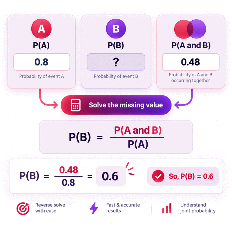
Suppose independent events have P(A∩B) = 0.18. You also know P(B) = 0.30. The missing P(A) can be found by division.
P(A) = P(A∩B) ÷ P(B)
P(A) = 0.18 ÷ 0.30
P(A) = 0.60
The result is 60%.
This reverse method is useful during audits. You can compare an implied input against the original data. If the implied probability seems impossible, the assumption may need review.
Finding a Conditional Probability From P(A and B)
Dependent events use the same idea with a conditional factor. Suppose P(A∩B) is 0.28 and P(B) is 0.40.
P(A|B) = P(A∩B) ÷ P(B)
P(A|B) = 0.28 ÷ 0.40
P(A|B) = 0.70
The conditional probability is 70%.
Why Division by Zero Creates an Undefined Reverse Problem
One edge case requires special care. If the divisor is zero, ordinary reverse solving cannot produce a unique probability.
Suppose P(B) equals zero. The joint event must also have zero probability under this model. If both are zero, many different values of P(A|B) could appear algebraically without changing the product. The missing factor is therefore not uniquely determined from those values.
A reliable calculator should report that limitation. It should not invent a number.
Why Can a Plausible-Looking Probability Still Be Impossible?
Numbers between zero and one can still contradict each other. This is one reason automatic validation matters.
Suppose P(A∩B) is 0.60 and P(B) is 0.40. Reverse solving would require the other factor to equal 1.50. A probability of 1.50 is impossible.
The problem is not the division. The known values violate the probability model.
Checking Whether the Joint Result Fits the Known Events
A joint event is more restrictive than either event alone. If both A and B must occur, every joint outcome belongs to A and also belongs to B.
That gives a useful check:
P(A∩B) cannot exceed P(A).
P(A∩B) cannot exceed P(B).
For the dependent orientation used by the calculator, P(A∩B) also cannot exceed P(B). The conditional factor is never greater than one.
Fast Sanity Checks Before You Trust the Result
First, check the event relationship. Second, check that every probability is within its valid scale. Third, confirm that percentages were not mistaken for decimals. Fourth, inspect the joint result against the known marginal probabilities.
These checks take seconds. They prevent many common errors.
How Should You Read P(A∩B), P(A and B), and Event Intersections?
Probability notation can make a simple idea look harder. P(A∩B) means the probability that both A and B occur. P(A and B) communicates the same idea in plain language.
The intersection symbol comes from set theory. Imagine all outcomes belonging to event A inside one circle. Put all outcomes belonging to B inside another. Their overlapping region contains outcomes satisfying both conditions.
What the Overlap in a Venn Diagram Actually Means
A Venn diagram is useful for understanding structure. The overlap shows where the two event sets intersect.
It does not automatically tell you the numerical probability. The probability still depends on the data or model.
This matters when people assume that a large-looking overlap means a large probability. Diagrams are conceptual. Calculations require measured, counted, or modeled probabilities.
Where Does Joint Probability Matter Outside the Classroom?
Joint probability becomes valuable whenever decisions depend on multiple conditions occurring together.
Risk Analysis and Reliability Decisions
A risk analyst may ask whether two failure conditions can occur in the same operating period. An engineer may study whether one condition changes the chance of another. The independence assumption then becomes crucial.
Multiplying unrelated failure probabilities may be reasonable in one model. It may be misleading when failures share a cause.
This is why the relationship between events matters more than the arithmetic itself.
Data Science, Experiments, and Predictive Models
Data analysis often studies combinations of observations. Joint probabilities can describe how variables occur together. Conditional probabilities then show how the distribution changes after information is known.
This distinction sits behind many statistical and predictive methods. The simple two-event calculator is therefore connected to much larger models.
Quality Control and Operational Decisions
A production team may track two defect conditions. Operations staff may study delays together with equipment states. A survey analyst may examine two responses occurring in the same record.
The numbers can guide investigation. They should not automatically be treated as proof of causation.
What Mistakes Produce the Largest Joint Probability Errors?
The largest errors often begin before a number is entered. A wrong assumption can produce perfectly executed arithmetic and a useless answer.
Multiplying Marginal Probabilities When Events Are Dependent
This is the central mistake. Two ordinary probabilities are multiplied even though one event changes the other.
The fix is simple. Use a relevant conditional probability for the dependent factor.
Another error occurs when the conditional direction is reversed. P(A|B) is not automatically equal to P(B|A). Always read the notation before using it.
Confusing Mutually Exclusive Events With Independent Events
These concepts describe different relationships.
Mutually exclusive events cannot both occur. Their intersection is zero. Independent events do not change each other’s probabilities.
If two ordinary events are mutually exclusive and one occurs, you immediately know the other did not occur. That is information. They are therefore not generally independent.
This distinction appears often in probability exercises and real classification problems.
How Can You Use AxiCalculator to Check a Joint Probability Faster?
Start by defining the events clearly. Do not enter numbers until you know what A and B represent.
Next, decide whether one event changes the probability of the other. Choose independent mode when it does not. Choose dependent mode when a conditional probability is required.
Enter any two valid known quantities. AxiCalculator can calculate the missing probability in the supported relationship. You can also edit the joint result and work backward.
Then perform a quick logic check. Confirm that each probability lies within the possible range. Check that the joint probability is not larger than a required marginal event. Review any reverse result that approaches zero or one.
The best use of a Joint Probability Calculator is not blind multiplication. It is structured verification.
That difference matters when a result will influence a report, assignment, experiment, risk assessment, or technical decision. A calculator should shorten the arithmetic while keeping the assumptions visible.
AxiCalculator is built around that workflow. Enter the known values, select the relationship, inspect the result, and reverse-check it when needed. A few seconds of validation can save much longer corrections later.
Frequently Asked Questions
Why can two reasonable probability inputs still produce a misleading joint result?
Does a low joint probability mean the individual events are unlikely?
Why does changing the order of conditional probability matter?
Can a Venn diagram calculate the exact joint probability by itself?
How should an engineer handle two failure events that may share one cause?
What should a data analyst do if reverse solving returns a probability above 100%?
Why is a zero probability difficult when solving a joint equation backward?
Our engineers are here to help you get it right.