Post-Test Probability Calculator
- Last formula update:

Decimal & Rounding Policy
- All probabilities are converted to decimal proportions before calculation.
- Intermediate calculations retain full floating-point precision and are never rounded early.
- Displayed probabilities and percentages use up to 6 decimal places with trailing zeros removed.
- Likelihood ratios and odds use up to 6 decimal places with trailing zeros removed.
- True positive, false positive, true negative, and false negative counts remain whole numbers.
- Reverse-solved counts are accepted only when the mathematical result is a valid whole number.
- Final rounding affects display only and never changes the underlying calculation state.
Valid range
- Pre-test probability: 0% to 100%; 100% is treated as a certainty boundary with infinite pre-test odds.
- Post-test probability: 0% to 100%; boundary values require mathematically valid finite or limiting inputs.
- Sensitivity: 0% to 100%, equivalent to a proportion from 0 to 1.
- Specificity: 0% to 100%, equivalent to a proportion from 0 to 1.
- Positive likelihood ratio: 0 or greater; mathematically valid cases may approach infinity.
- Negative likelihood ratio: 0 or greater; mathematically valid cases may approach infinity.
- Pre-test odds: 0 or greater; probability equal to 100% corresponds to infinite odds.
- Post-test odds: 0 or greater; probability equal to 100% corresponds to infinite odds.
- TP, TN, FP, and FN: non-negative whole-number counts only.
- Confusion-matrix counts must produce nonzero denominators for every requested derived metric.

Wylena Brantford
Reviewers:
Valdren Clyforde
Zenara Dentwick
Check our editorial policy
September 14, 2026
1.0.0
Initial calculator and formula release.
Our engineers are here to help you get it right.
How Does a Post-Test Probability Calculator Update Diagnostic Probability?
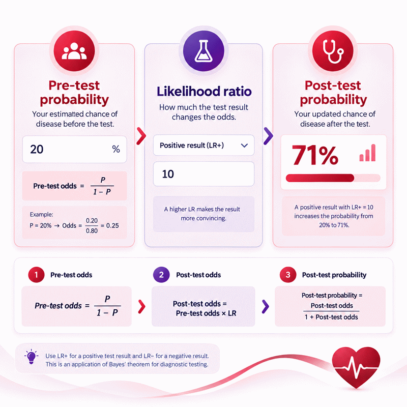
Post-Test Probability Calculator results show how a diagnostic test changes an existing estimate of a condition after new evidence becomes available. The calculator starts with the pre-test probability, applies the likelihood ratio associated with the observed result, and returns the updated post-test probability in a clear Bayesian workflow.
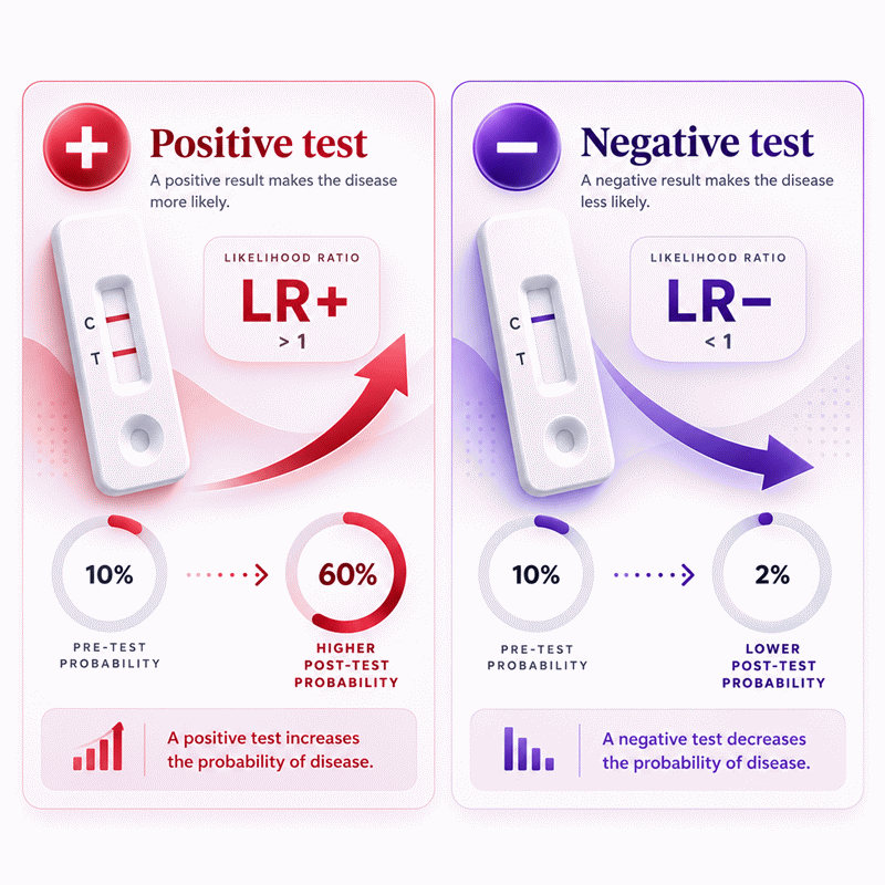
- Use LR+ when the observed diagnostic result is positive.
- Use LR− when the observed diagnostic result is negative.
- The same test can produce different outcomes at different starting probabilities.
- Prevalence can provide a starting estimate when it matches the tested population.
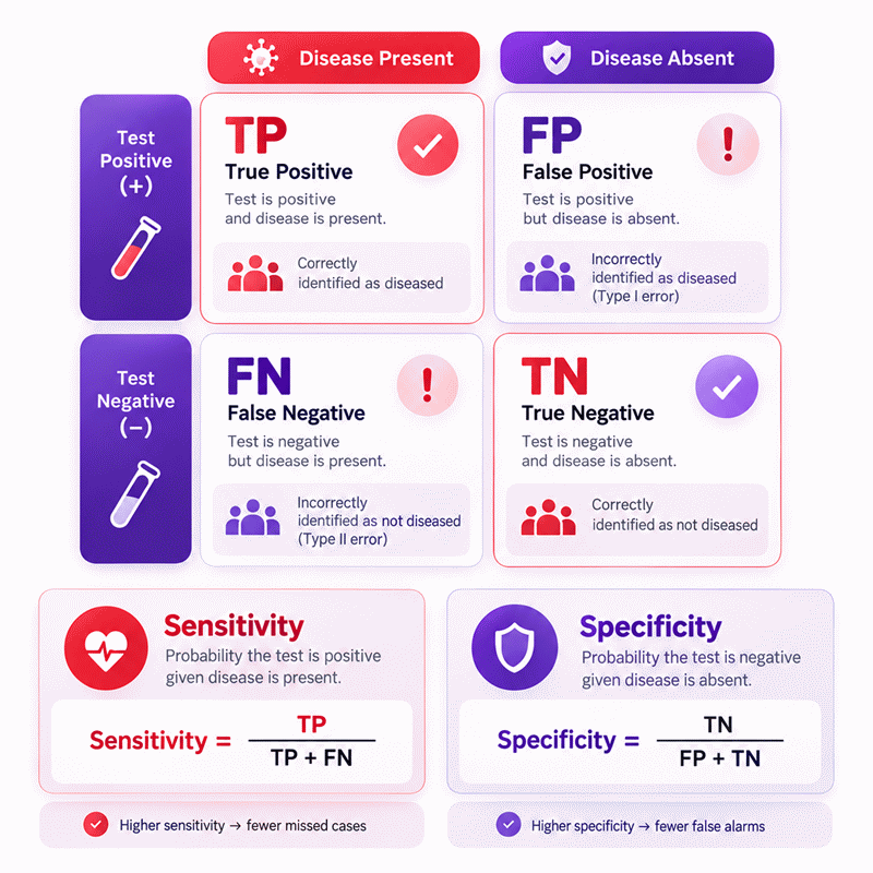
- Sensitivity and specificity can be used to derive likelihood ratios.
- TP, FP, TN, and FN data can support diagnostic-performance calculations.
- Reverse solving can recover a missing likelihood ratio or starting probability.
- Values near LR = 1 create little change in diagnostic probability.
- Extreme probabilities and extreme test metrics require careful interpretation.
A Post-Test Probability Calculator is most useful when the starting probability, test characteristics, and result direction are defensible. The final percentage should be interpreted as an evidence update rather than a stand-alone diagnosis.
Assumptions used in this calculator
- Pre-test probability represents the relevant population or individualized prior probability.
- Selected likelihood ratio matches the observed test result.
- Sensitivity and specificity apply to the tested population and threshold.
- True and false counts are correctly classified and mutually exclusive.
- Count inputs represent the same study population and time frame.
- Probability inputs are converted consistently between percent and proportion.
- Likelihood ratios are nonnegative and dimensionless.
- Intermediate calculations retain full precision before final display rounding.
- Reverse calculations require mathematically identifiable, nondegenerate input combinations.
- Extreme probabilities may produce infinite odds or boundary results.
- Missing, invalid, or incompatible inputs are excluded from calculation.
- Clinical interpretation depends on context, prevalence quality, and test validity.
- Calculator outputs support decision analysis, not standalone medical diagnosis.
Results are rounded for display.
Internal calculations use full precision.
Formulas Used in Post-Test Probability Calculator :
Probability Unit Normalization
Sensitivity
Specificity
Positive Likelihood Ratio
Negative Likelihood Ratio
Pre-Test Probability from Diagnostic Counts
Pre-Test Odds
Post-Test Odds
Post-Test Probability
Reverse Solving
- TP — true positive count.
- FN — false negative count.
- TN — true negative count.
- FP — false positive count.
- Se — sensitivity expressed as a proportion.
- Sp — specificity expressed as a proportion.
- LR+ — positive likelihood ratio.
- LR− — negative likelihood ratio.
- LR — likelihood ratio selected for the observed test result.
- P — pre-test probability or prevalence expressed as a proportion.
- P% — pre-test probability expressed as a percentage.
- Opre — pre-test odds.
- Opost — post-test odds.
- Q — post-test probability expressed as a proportion.
Variables & Definitions
View a complete list of all variables used in this calculator, including definitions and units
Post-Test Probability Calculator Variables and Definitions
| Variable | Name | Valid Range | Unit | Used For |
|---|---|---|---|---|
| TP | True Positive | Non-negative whole number | Cases | Sensitivity and prevalence |
| FN | False Negative | Non-negative whole number | Cases | Sensitivity and prevalence |
| TN | True Negative | Non-negative whole number | Cases | Specificity and prevalence |
| FP | False Positive | Non-negative whole number | Cases | Specificity and prevalence |
| Se | Sensitivity | 0 to 1 | Proportion or % | Positive and negative likelihood ratios |
| Sp | Specificity | 0 to 1 | Proportion or % | Positive and negative likelihood ratios |
| LR+ | Positive Likelihood Ratio | 0 to infinity | Dimensionless | Positive test-result updating |
| LR− | Negative Likelihood Ratio | 0 to infinity | Dimensionless | Negative test-result updating |
| LR | Selected Likelihood Ratio | 0 to infinity | Dimensionless | Converting pre-test odds into post-test odds |
| P | Pre-Test Probability | 0 to 1 | Proportion or % | Starting probability before the test result |
| P% | Pre-Test Probability Percentage | 0% to 100% | % | User-facing percentage representation of P |
| Opre | Pre-Test Odds | 0 to infinity | Dimensionless | Bayesian odds update |
| Opost | Post-Test Odds | 0 to infinity | Dimensionless | Converting the updated odds into probability |
| Q | Post-Test Probability | 0 to 1 | Proportion or % | Final probability after applying the test result |
Unit Conversion Table
Probability Units
| Unit Group | Unit Name | Symbol | Equivalent in Proportion | Used For |
|---|---|---|---|---|
| Popular Units | Percent | % | 1% = 0.01 | Pre-test probability, post-test probability, sensitivity, specificity |
| Scientific Units | Proportion | 1 | 1 = 1 | Internal probability calculations and scientific notation |
Dimensionless Ratio Units
| Unit Group | Unit Name | Symbol | Equivalent in Base Ratio | Used For |
|---|---|---|---|---|
| Scientific Units | Dimensionless Ratio | 1 | 1 ratio unit = 1 | LR+, LR−, selected likelihood ratio, pre-test odds, post-test odds |
Diagnostic Count Units
| Unit Group | Unit Name | Symbol | Equivalent in Cases | Used For |
|---|---|---|---|---|
| Popular Units | Case Count | cases | 1 case = 1 case | TP, TN, FP, and FN diagnostic counts |
Example Calculation
Selected likelihood ratio = 7.5
P = 18 / 100 = 0.18
Opre = 0.18 / (1 − 0.18) = 0.2195121951
Opost = 0.2195121951 × 7.5 = 1.6463414634
Q = 1.6463414634 / (1 + 1.6463414634) = 0.6221198157
The calculation begins with an 18% probability before the test result is considered.
Converting probability to odds creates the form required for likelihood-ratio updating.
Applying a likelihood ratio of 7.5 substantially increases the odds of the condition.
The updated odds correspond to a final post-test probability of approximately 62.212%.
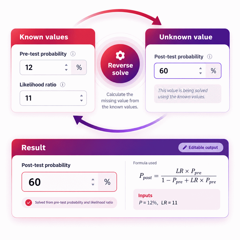
Known post-test probability = 60%
Unknown likelihood ratio = ?
P = 0.12
Q = 0.60
Opre = 0.12 / (1 − 0.12) = 0.1363636364
Opost = 0.60 / (1 − 0.60) = 1.5
LR = Opost / Opre
LR = 1.5 / 0.1363636364 = 11
The reverse calculation starts with the known probabilities before and after testing.
Both probabilities are converted into odds so the likelihood ratio can be isolated.
A likelihood ratio of 11 changes a 12% pre-test probability to exactly 60%.
This reverse mode is useful when the required diagnostic evidence strength is unknown.
Results are rounded for display.
Internal calculations use full precision.
Calculations Disclaimer
What Does a Post-Test Probability Calculator Tell You After a Test?
A test result can look decisive while still leaving an important question unanswered: how likely is the condition now? A Post-Test Probability Calculator answers that question by connecting what was believed before the test with the strength of the evidence delivered by the result. Instead of treating a result as a simple yes-or-no verdict, it shows how much the probability actually moved.
This distinction matters because diagnostic tests do not operate in isolation. The meaning of a result depends on the situation before testing. A positive result in a low-risk setting may produce a very different conclusion from the same positive result in a high-risk setting. A negative result can also reduce probability dramatically in one case but leave substantial uncertainty in another.
The calculator therefore works best as an evidence-update tool. It helps students understand Bayesian reasoning, researchers review diagnostic performance, and professionals examine how a test result changes an existing estimate. The useful output is not only the final percentage. The real value is the movement between the starting and updated probabilities.
AxiCalculator keeps that movement visible. You can enter the information you know, review the updated value immediately, and change an assumption to see how strongly it affects the result. This turns a concept that often feels abstract into an interactive decision workflow.
Why Can the Same Test Result Produce a Different Probability for Two People?
Two people can receive the same test result and still finish with very different probabilities. The reason is simple but easy to overlook: they may not have started at the same probability. A test updates existing information; it does not erase the information that was already available.
Imagine one situation where the condition is uncommon and there are few reasons to suspect it. The starting probability is low. Now consider another situation where symptoms, exposure, previous findings or a high-risk setting make the condition much more plausible before testing. The same diagnostic evidence is being applied to two very different starting points.
This is why an isolated statement such as “the test is highly accurate” is not enough to understand an individual result. The relevant question is how strongly the observed result changes the probability that existed before the test. A useful calculator keeps that starting estimate visible instead of hiding it behind the final number.
This also explains why comparing final probabilities across unrelated populations can be misleading. The difference may come from the starting risk rather than from a better or worse test. Good diagnostic reasoning separates these effects before drawing conclusions.
Pre-Test Probability Sets the Starting Point Before New Evidence Arrives
A common mistake begins before the calculation even starts: the user enters a pre-test probability without asking what it represents. That value is the foundation of the entire update, so its relevance matters as much as the mathematics that follows.
Pre-test probability describes the estimated chance of the condition before the new result is incorporated. Depending on the context, that estimate can come from population frequency, a validated risk model, previous evidence or a carefully justified professional assessment. The best source is the one that most closely represents the actual situation being evaluated.
If the starting estimate is unrealistically low, the updated probability may be misleadingly low. If it is exaggerated, the final value may appear much more convincing than the evidence supports. Changing the starting probability is therefore not a cosmetic adjustment. It changes the entire interpretation.
A useful workflow records the starting estimate explicitly. That makes the calculation easier to reproduce, audit and discuss with another person.
Population Prevalence and Individual Clinical Probability Are Not Always Identical
A population prevalence figure is convenient, but convenience can hide a mismatch. A person entering a diagnostic pathway may not resemble the general population from which the prevalence estimate was taken.
Prevalence describes how common a condition is within a defined population. Individual pre-test probability may incorporate additional information that was already known before the new test. Symptoms, previous screening, referral patterns, age group, exposure and selection criteria can all create a population whose starting risk differs from a broad community average.
This does not mean prevalence is useless. It can be a reasonable prior estimate when the population and use case match. The problem begins when a broad prevalence value is treated as universally applicable.
For reliable interpretation, ask a practical question before entering the number: does this starting probability represent the people or situation being evaluated? If the answer is uncertain, the output should be treated with the same uncertainty.
Which Likelihood Ratio Should You Use for the Result You Actually Received?
A calculation can be numerically perfect and conceptually wrong if the wrong likelihood ratio is applied. The likelihood ratio must correspond to the result that was actually observed.
A positive result normally uses the positive likelihood ratio. A negative result normally uses the negative likelihood ratio. These two values describe different evidence directions, so they should not be swapped simply because they come from the same diagnostic test.
This is particularly important when a user copies performance data from a paper or report. Sensitivity, specificity, positive likelihood ratio and negative likelihood ratio may all appear together. The calculator needs the value associated with the observed result.
When test results have more than two categories, a result-specific likelihood ratio can sometimes be more informative than forcing the result into a simple positive or negative group. The central rule remains the same: apply evidence that matches what was actually observed.
How LR+ Changes Diagnostic Confidence After a Positive Result
A positive result can create instant confidence, but the size of that confidence should depend on how informative the result actually is. LR+ expresses how strongly a positive result supports the presence of the condition relative to its absence.
Values close to one produce little change. Larger values create a stronger upward shift in the odds. However, even a strong LR+ cannot be interpreted without the starting probability. A rare condition can remain far from certain after a positive result, while the same evidence can create a much higher final probability in a high-risk setting.
This is why a calculator should show the probability before and after the test. The comparison makes the evidence contribution visible. It also prevents users from confusing a positive test result with certainty.
The practical question is not merely “Was the result positive?” It is “How much evidence did this positive result add?”
How LR− Changes Diagnostic Confidence After a Negative Result
A negative result often creates relief, but relief is not the same as a sufficiently low probability. LR− describes how strongly the negative result shifts evidence away from the condition.
A value close to one has little effect. A much smaller value can sharply reduce the odds. Yet the remaining probability still depends on where the calculation began. A negative result that is reassuring in a low-risk case may leave significant uncertainty in a high-risk case.
This is especially important when the consequences of a missed condition are serious. The calculator can quantify the statistical change, but the threshold for taking further action is determined by the real decision context.
For clear interpretation, compare the starting and final probabilities rather than treating the word “negative” as the conclusion.
How Sensitivity and Specificity Shape the Evidence Behind a Test Result
Users often know sensitivity and specificity but do not know how those values affect the probability they care about. Sensitivity describes how often the test identifies the condition when it is present. Specificity describes how often the test correctly produces a negative result when the condition is absent.
These measures help characterize a diagnostic test, but they answer different questions from the one faced after a result is observed. The likelihood ratios connect these performance characteristics with the probability-update process.
High sensitivity can make negative results more informative when false negatives are uncommon. High specificity can make positive results more informative when false positives are uncommon. The balance matters because no single percentage captures every diagnostic property.
When sensitivity and specificity are entered into a calculator, they should come from evidence that matches the relevant test method, threshold and population as closely as possible. A technically impressive performance figure from a very different setting may not transfer perfectly.
Why False Positives Matter When Specificity Falls
A positive result may look alarming until the false-positive behavior of the test is considered. Lower specificity means more people without the condition can still receive a positive result.
This becomes particularly important when the condition is uncommon. If most tested people do not have the condition, even a modest false-positive rate can generate a meaningful number of positive results among people who are actually condition-free.
The implication is not that the test is useless. It means the positive result must be interpreted together with its likelihood ratio and the starting probability. A transparent calculator makes that relationship visible instead of encouraging a binary interpretation.
When a surprising positive result appears in a low-risk context, the right next question is about evidence strength, not certainty.
Why False Negatives Matter When Sensitivity Falls
A negative result may appear reassuring even when the test misses a meaningful share of true cases. Lower sensitivity increases the possibility that people with the condition receive a negative result.
This matters most when the starting probability is already substantial. A weak negative result may reduce probability without reducing it enough to change the practical decision.
The correct interpretation therefore depends on both the test’s ability to detect true cases and the starting level of concern. Looking only at the word “negative” hides both pieces of information.
A good calculator helps expose this issue by showing how far the probability actually moved. If the shift is small, the negative result should not be treated as more informative than it really is.
What Happens to Probability After a Positive Diagnostic Test?
A positive test result creates a natural urge to jump directly to the final probability. That shortcut hides the most informative part of the process: the amount of change created by the test.
The starting probability is first converted into a form that can be updated by diagnostic evidence. The likelihood ratio then changes that evidence state, and the updated value is converted back into a probability that is easier to interpret.
The final number can rise slightly or dramatically. The size of that increase depends on both the initial probability and the strength of the positive evidence. This is why a moderately informative positive result can be powerful in one setting and much less decisive in another.
When reviewing the result, look at the before-and-after comparison. The difference tells you what the test actually contributed. A large final probability does not necessarily mean the test alone was powerful; the starting probability may already have been high.
What Happens to Probability After a Negative Diagnostic Test?
A negative test result can reduce uncertainty, but the remaining risk is what matters. The calculator applies the evidence associated with the negative result to the starting probability and reports the updated probability.
If the negative evidence is strong, the result can move sharply downward. If it is weak, the change may be small. The same negative test can therefore produce different practical interpretations depending on the person or population being evaluated.
This matters in screening, triage and follow-up decisions. A low starting probability combined with strong negative evidence can leave very little residual probability. A high starting probability combined with weak negative evidence may still leave enough uncertainty to justify further assessment.
The calculator quantifies the update. The practical decision must still consider the consequences of acting, waiting or obtaining more information.
Why Low Prevalence Can Make a Positive Result Less Convincing Than Expected
A rare condition creates a statistical trap: even an apparently strong test can produce a positive result that is less conclusive than intuition expects. The reason is the large number of people who begin without the condition.
When the starting probability is very low, the diagnostic evidence must overcome a substantial prior imbalance. A positive result can increase the probability many times while the final value still remains far below certainty.
This effect is one reason population screening requires careful interpretation. A percentage describing test performance cannot be read in isolation from the frequency of the condition in the tested population.
The practical advantage of a Post-Test Probability Calculator is that it makes this interaction visible instantly. Change the starting probability while keeping the test evidence constant, and the final result can move substantially.
Why High Pre-Test Probability Can Survive a Negative Test Result
A negative result can feel decisive even when the condition was highly plausible before testing. If the starting probability is high, weak or moderate negative evidence may not reduce it enough to remove concern.
This is the mirror image of the low-prevalence positive-test problem. The prior information matters. A diagnostic result updates that information rather than replacing it.
When the consequences of a missed condition are serious, this distinction becomes especially important. A statistically meaningful reduction may still leave a probability that requires action.
The calculator should therefore be used to answer “How much did the negative result change the situation?” rather than “Did the negative result prove absence?”
When Can Post-Test Probability Become Misleading?
A mathematically correct result can still mislead when the inputs do not represent the real situation. The most common problem is not arithmetic; it is input quality and transferability.
A pre-test probability may come from an unsuitable population. Test characteristics may come from a different threshold or patient spectrum. A likelihood ratio may be copied without confirming whether it belongs to a positive, negative or result-specific category.
Another problem appears when a precise-looking output hides uncertain evidence. A final percentage with several decimal places does not become scientifically stronger simply because it is displayed precisely.
The safest approach is to treat the calculator as a transparent transformation of the supplied evidence. Better inputs produce more meaningful outputs. Weak inputs remain weak even when the arithmetic is flawless.
Population Spectrum Can Change Real-World Test Performance
A diagnostic study may contain patients who are very different from the people being evaluated later. Disease severity, comorbidities, age, referral patterns and competing conditions can change how easy the condition is to distinguish.
This is often called a spectrum issue. A test that performs very well in a highly selected validation group may perform differently in broader routine use.
The practical lesson is to look beyond the headline sensitivity or specificity. Ask whether the study population resembles the intended use population. If not, the resulting likelihood ratio may not transfer perfectly.
The calculator cannot repair a mismatch in evidence. It can only update probability using the values supplied.
Diagnostic Thresholds Can Shift Sensitivity, Specificity and Likelihood Ratios
Many diagnostic measurements are continuous, but a positive or negative label is created by choosing a threshold. Changing that threshold can change which cases are classified as positive and negative.
A more permissive threshold can increase sensitivity while reducing specificity. A stricter threshold may do the opposite. Because likelihood ratios depend on these characteristics, the evidence associated with a test result can also change.
This means a likelihood ratio should be linked to the correct method and threshold. Using a value from a different cutoff can make the final probability look authoritative while representing the wrong diagnostic rule.
Whenever possible, document the test definition behind the LR rather than treating the number as universally portable.
Small Validation Samples Can Make Extreme Test Metrics Look Stronger Than They Are
A small validation study can produce perfect-looking sensitivity or specificity simply because no error happened to appear in a limited sample. That does not guarantee the same performance in a larger population.
Extreme values can produce extreme likelihood ratios. The mathematical result may be correct for the observed table, but uncertainty around the estimate can still be large.
This is why test-performance evidence should be evaluated with sample size and uncertainty in mind. A point estimate is only one part of the picture.
For professional interpretation, the confidence placed in the final post-test probability should reflect the confidence placed in the inputs.
How Does Reverse Solving Help With Diagnostic Planning?
Sometimes the missing value is not the post-test probability. A researcher may know the starting probability and a desired target probability but want to know how strong the diagnostic evidence must be to reach that target.
Reverse solving turns the calculator into a planning tool rather than a one-direction answer box. It can also recover a starting probability when the likelihood ratio and resulting probability are known.
This capability is useful for education, scenario analysis and study planning because it exposes the relationship between the variables from another direction. It makes the calculator behave like a connected mathematical system rather than a simple input-output form.
The important condition is that the known values must define a unique, valid solution. Boundary cases can become undefined or non-unique, so a robust implementation should reject those combinations instead of inventing an answer.
How to Find the Required Likelihood Ratio From a Target Probability
A target probability can be useful when asking what strength of evidence would be required to move from a known starting point to a specified updated level. Reverse solving isolates the likelihood ratio that would create that change.
This does not mean the required LR automatically exists in the real world. It describes a mathematical requirement. The next task is to determine whether a real diagnostic test or finding can provide evidence of that strength in the relevant population.
This distinction prevents scenario planning from becoming a false clinical claim. The calculator tells you what the relationship requires; evidence tells you whether that requirement is realistic.
How to Recover the Starting Probability From a Known Result
A different reverse problem appears when the final probability and likelihood ratio are known but the original starting probability is missing. The Bayesian relationship can be solved backward to recover the prior estimate.
This is useful when auditing a published calculation or reconstructing a scenario. If the recovered starting value looks implausible, that can reveal an incorrect LR, a transcription error or a mismatch in assumptions.
Reverse calculation therefore does more than fill a blank field. It provides another way to test whether the numbers are internally consistent.
How Should Students, Researchers and Professionals Interpret the Final Probability?
A final percentage can look like a verdict, but it is better understood as the output of a defined evidence model. It answers a statistical question using the starting probability and diagnostic evidence supplied by the user.
Students can use the result to understand how Bayes-style updating works. Researchers can use it to explore the implications of reported test performance. Professionals can use it as one transparent quantitative component within a broader decision process.
The strongest interpretation always includes context. State the starting probability, identify the evidence used, and report the updated probability. That makes the reasoning reproducible and avoids presenting an isolated number as if it appeared from nowhere.
A good result is not merely numerically correct. It should also be understandable, traceable and appropriately limited.
Use the Result as an Evidence Update Rather Than a Binary Verdict
Real decisions rarely become simple just because a probability has been calculated. The updated value may cross a practical action threshold, remain in an uncertain middle region, or suggest that more evidence is needed.
The calculator cannot define one universal threshold because the consequences of errors differ between contexts. Missing a serious condition may carry a very different cost from performing an unnecessary follow-up test.
The most useful interpretation is therefore directional and contextual. Ask how far the evidence moved the probability and whether that movement is enough to change the next decision.
How Can AxiCalculator Make Bayesian Diagnostic Reasoning Faster and Easier to Audit?
Many probability tools return one number and hide the path that produced it. AxiCalculator can be more useful by keeping the connected values visible and allowing the user to work in either direction.
Real-time calculation makes scenario testing fast. Reverse solving makes missing-variable problems practical. Visible intermediate values make the logic easier to check. Export and sharing functions make the same setup easier to reproduce with another person.
The interface should remain compact because diagnostic reasoning is already cognitively demanding. Every field needs a purpose. Every result should connect clearly to an entered or derived value.
The goal is not to make the mathematics look impressive. It is to make the reasoning understandable. When users can see what changed, why it changed and which assumption caused the movement, a calculator becomes more than an answer generator. It becomes a transparent analytical tool.
Frequently Asked Questions
Why can two people with the same positive test have different post-test probabilities?
Is post-test probability the same as the chance that a positive result is correct?
Why doesn't an LR of 1 change the result?
Should I use population prevalence as my pre-test probability?
Can I multiply likelihood ratios from several diagnostic tests?
How should I interpret an infinite LR+ or an LR− of zero?
When is reverse solving useful in diagnostic analysis?
Our engineers are here to help you get it right.