Cell Doubling Time Calculator

Last formula update: August 29, 2026

Trusted Engineering Tools

Calculate cell doubling time, growth rate, and missing culture parameters in seconds with a fast, flexible reverse-solving calculator. Enter your available measurements, switch units freely, and get clear results for cell growth analysis, experiment planning, and laboratory workflows.

Initial reference parameter

Final reference parameter

Time duration

Growth rate

Doubling time

Decimal & Rounding Policy

The Cell Doubling Time Calculator keeps full numerical precision during all intermediate calculations, including logarithms, growth rate, and doubling time.
Intermediate values are never rounded; rounding is applied only when the final result is displayed to the user.
Displayed results use practical significant digits and remove unnecessary trailing zeros for clear, readable values.
Very small or very large results may use scientific notation to preserve accuracy and readability.
Unit conversions are performed before final formatting, preventing cumulative rounding errors when switching between time or growth-rate units.
Small differences may appear when a rounded displayed result is manually reused because the calculator internally retains higher precision.

Valid range

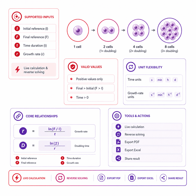
Initial reference parameter: enter a finite positive value greater than 0 and up to 1e300.
Final reference parameter: enter a finite positive value greater than the initial reference parameter and up to 1e300.
Time duration: enter a value greater than 0 and within the supported equivalent range of up to 1e12 hours.
Growth rate: valid exponential cell growth requires a positive rate greater than 0 and up to 1e12 h^-1.
Doubling time: the calculated or entered value must be finite and greater than 0, with a supported equivalent range of up to 1e12 hours.
The calculator applies the exponential growth relationship consistently, so zero, negative, non-finite, or mathematically incompatible values are rejected.

Creators

Olivara Dremmont

Reviewers:

Urellyn Vexmere

Ralven Pexthorne

Check our editorial policy

Formula Implementation date:

August 29, 2026

Formula Version:

1.0.0

Changelog:

Version 1.0.0

Initial calculator and formula release.

Need help selecting or validating calculations?

Our engineers are here to help you get it right.

How Does the Cell Doubling Time Calculator Turn Cell Culture Measurements Into Reliable Growth Insight?

Cell Doubling Time Calculator converts comparable cell culture measurements into a clear estimate of population growth. It uses the initial reference value, final reference value, and elapsed time to describe exponential growth. The Cell Doubling Time Calculator can also work in reverse, allowing a missing initial value, final value, time duration, growth rate, or doubling time to be solved when enough independent information is available.

Use the same measurement type for initial and final reference values.
Choose measurements from a period that reasonably reflects exponential population growth.
Interpret shorter doubling times as faster net population expansion under comparable conditions.
Review culture conditions, viability, density, or measurement quality when results change unexpectedly.
Use reverse solving for target populations, starting values, or expected culture duration.
Compare results only when experimental conditions and measurement methods remain consistent.
Check unusual results against culture history instead of relying on one calculation.

The result is most useful as a practical growth estimate, not a fixed biological property. Cell behavior can change with passage history, density, nutrients, stress, viability, and other culture conditions. For reliable decisions, combine the calculated result with direct observations and repeat measurements across repeated culture runs.

Assumptions used in this calculator

Cell populations are assumed to grow exponentially during the measured interval.
The growth rate is assumed constant throughout the selected time period.
Initial and final values represent the same biological measurement type.
Initial and final measurements are assumed accurate and experimentally comparable.
The final reference value must exceed the initial reference value.
Elapsed time is assumed positive and measured between corresponding observations.
Time units are assumed correctly selected before performing any calculation.
Growth rate and doubling time follow a continuous exponential growth model.
Environmental conditions are assumed sufficiently stable during the observation period.
Cell loss, contamination, and measurement artifacts are assumed clinically insignificant.
Culture conditions are assumed not to introduce major growth-phase transitions.
Calculated doubling time represents an estimate, not a guaranteed biological outcome.
Critical laboratory or industrial decisions require independent experimental verification.

Results are rounded for display.
Internal calculations use full precision.

Formulas Used in Cell Doubling Time Calculator :

Growth Rate

r = \frac{\ln (\frac{F}{I})}{t}

Doubling Time

D = \frac{\ln (2)}{r}

Variables

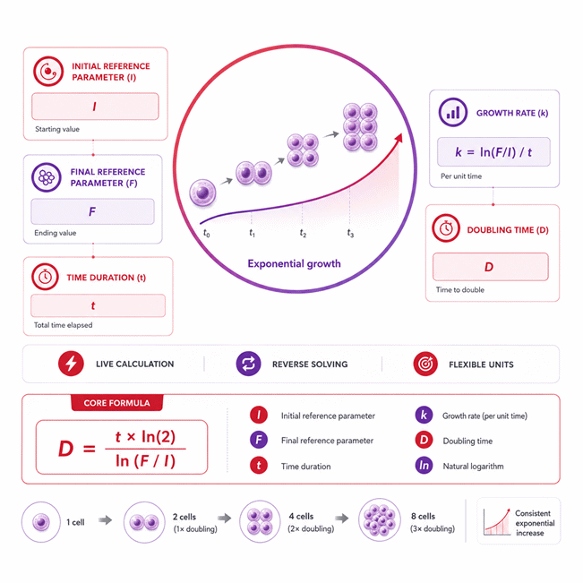
I = initial reference parameter, measured as a consistent cell count, concentration, confluency, or equivalent reference value.
F = final reference parameter, measured using the same reference type and scale as I.
t = elapsed time between the initial and final measurements.
r = exponential growth rate expressed as the reciprocal of the selected time unit.
D = cell doubling time expressed in the same time dimension as t.
ln = natural logarithm.

The calculator first determines the exponential growth rate and then calculates the doubling time. Reverse calculations use algebraic rearrangement of these same independent relationships without introducing additional formulas. Time values are converted to a consistent internal time basis before calculation, and growth-rate units use the corresponding reciprocal time basis.

Variables & Definitions

View a complete list of all variables used in this calculator, including definitions and units

Cell Doubling Time Calculator Variables and Parameters

Symbol	Variable	Description	Unit	Calculation Role
I	Initial reference parameter	The measured cell reference value at the beginning of the observation period.	Same reference unit as F	Initial value used to determine relative population growth.
F	Final reference parameter	The measured cell reference value at the end of the observation period.	Same reference unit as I	Final value used to determine relative population growth.
t	Time duration	The elapsed time between the initial and final reference measurements.	s, min, h, or d	Defines the time interval over which exponential growth is measured.
r	Growth rate	The exponential growth rate calculated from the change in the reference parameter over time.	s^-1, min^-1, h^-1, or d^-1	Links the measured population change to the cell doubling time.
D	Doubling time	The estimated time required for the cell reference parameter to increase by a factor of two.	s, min, h, or d	Represents the primary cell doubling time result.
ln	Natural logarithm	The logarithmic operation with base e used in the exponential growth calculation.	Dimensionless	Transforms the relative change between F and I for growth-rate calculations.

Unit Conversion Table

Cell Doubling Time and Growth Rate Unit Conversion Table

Unit Group	Unit Name	Symbol	Equivalent in Base Unit	Used For
Popular Units	Hour	h	1 h	Time duration and doubling time
Popular Units	Minute	min	1 min = 1/60 h	Time duration and doubling time
Popular Units	Day	d	1 d = 24 h	Time duration and doubling time
Scientific Units	Second	s	1 s = 1/3600 h	Time duration and doubling time
Popular Units	Per Hour	h^-1	1 h^-1	Growth rate
Popular Units	Per Minute	min^-1	1 min^-1 = 60 h^-1	Growth rate
Popular Units	Per Day	d^-1	1 d^-1 = 1/24 h^-1	Growth rate
Scientific Units	Per Second	s^-1	1 s^-1 = 3600 h^-1	Growth rate

Example Calculation

Initial reference parameter 12,500 cells/mL

Final reference parameter 50,000 cells/mL

Time duration 60 h

Formula

D = t × ln(2) ln(F / I)

Solution

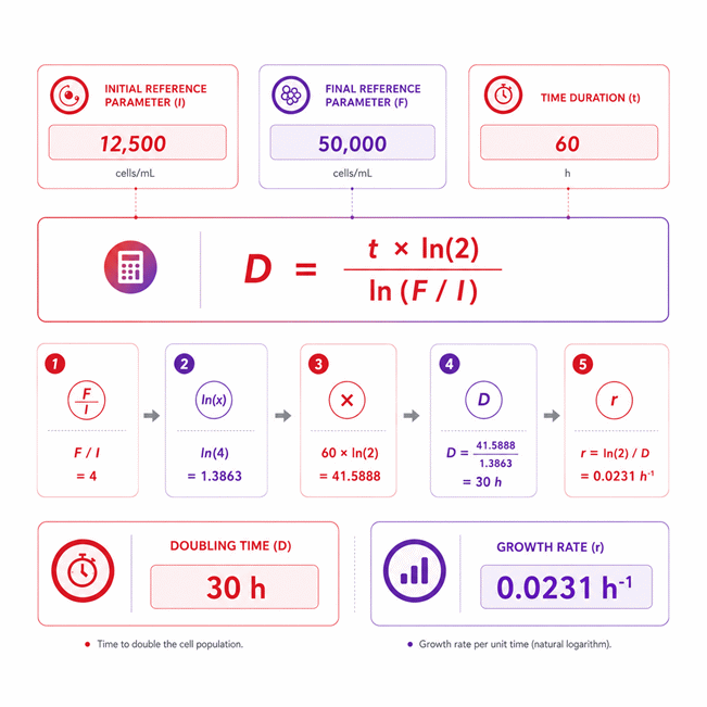
F / I = 50,000 / 12,500 = 4
ln(4) = 1.38629436112
60 × ln(2) = 60 × 0.69314718056 = 41.5888308336
D = 41.5888308336 / 1.38629436112 = 30 h
r = ln(4) / 60 = 0.023104906 h^-1

Doubling time 30 h

Growth rate 0.023104906 h^-1

The reference parameter increases from 12,500 to 50,000 cells/mL in 60 hours. This is a fourfold increase, corresponding to two complete population doublings. The calculated doubling time is therefore 30 hours under the assumed exponential growth conditions. The growth rate represents the continuous exponential rate associated with the same measurements.

Calculation Relationships

r = ln(F / I) t

D = ln(2) r

F = I × e^rt

I = F × e^-rt

t = ln(F / I) r

r = ln(2) D

Initial reference parameter 18,000 cells/mL

Time duration 48 h

Doubling time 24 h

Formula

r = ln(2) D

F = I × e^rt

Solution

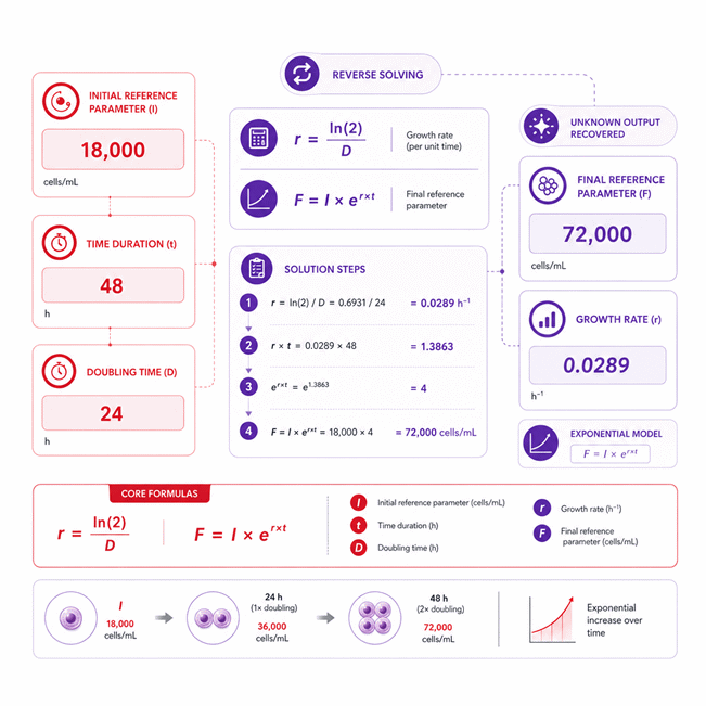
r = ln(2) / 24 = 0.69314718056 / 24
r = 0.0288811325 h^-1
r × t = 0.0288811325 × 48 = 1.38629436112
F = 18,000 × e^{1.38629436112}
F = 18,000 × 4 = 72,000 cells/mL

Calculated final reference parameter 72,000 cells/mL

Calculated growth rate 0.0288811325 h^-1

The initial reference parameter is 18,000 cells/mL and the doubling time is 24 hours. Over a 48-hour interval, the population completes two doubling periods. Reverse solving first determines the exponential growth rate and then calculates the unknown final reference parameter. The resulting final value is 72,000 cells/mL under constant exponential growth conditions.

Reverse Calculation Relationships

r = ln(F / I) t

D = ln(2) r

r = ln(2) D

F = I × e^rt

I = F × e^-rt

t = ln(F / I) r

t = D × ln(F / I) ln(2)

Results are rounded for display.
Internal calculations use full precision.

Calculations Disclaimer

Read important information about accuracy, limitations and responsible use of this calculator

This Cell Doubling Time Calculator provides mathematical estimates based on an exponential growth model using the initial reference parameter, final reference parameter, elapsed time, growth rate, and doubling time. Results assume that the selected cell population grows at an approximately constant exponential rate during the measured period. Actual biological growth may vary because of cell type, nutrient availability, temperature, culture conditions, confluency, experimental technique, measurement accuracy, and changes between growth phases. Calculator results are intended for educational, laboratory planning, and analytical purposes and should not replace validated experimental measurements, laboratory protocols, professional scientific judgment, or clinical decision-making. Always verify important results with appropriate laboratory methods and use consistent reference parameters and units throughout the calculation.

How Does a Cell Doubling Time Calculator Turn Culture Data Into a Useful Result?

A cell culture team often has several measurements but needs one clear answer. The Cell Doubling Time Calculator turns those measurements into an easy growth estimate. The Cell Doubling Time Calculator also supports reverse solving when one value is unknown. This matters when the experiment does not follow a perfect forward workflow.

The calculator works best when the measurements describe the same growing population. It reads the change between two observations and links that change to elapsed time. The result helps users judge how quickly the measured population expanded.

This process sounds simple, but poor input choices can distort the result. The most important work happens before any number is entered. Good measurements lead to useful output. Weak measurements produce a precise-looking number with little biological value.

Why Measurement Timing Changes the Meaning of the Result

A common problem starts when two measurements come from different growth phases. Cells may adapt slowly after seeding. They may later grow rapidly. They may also slow as space becomes limited.

A single result can hide these changes. For this reason, measurements should describe one reasonably stable growth period.

Choose a Consistent Growth Window

The safest window is usually a period of clear population expansion. The population should not be strongly limited by space or resources. Both measurements should also reflect similar culture conditions.

The goal is not to find the longest possible interval. The goal is to find a representative interval.

Avoid Combining Unrelated Culture Phases

A measurement taken soon after seeding may reflect adaptation. A later measurement may reflect rapid proliferation. Combining both can create an average that represents neither phase well.

This issue becomes more important in sensitive cultures. It also matters when passage conditions change between experiments.

Why the Same Measurement Method Matters

Users sometimes compare a starting cell count with a later confluency value. Those values describe different things. Their numerical ratio can therefore become misleading.

The starting and ending values should use the same measurement method. Cell count should be compared with cell count. Concentration should be compared with concentration. A consistent optical signal may also work when it remains proportional to population size.

Consistency matters more than the absolute scale.

A culture measured at 20,000 and 80,000 cells uses comparable data. The same principle applies to any other valid reference signal.

Quick visual check: Same culture → Same measurement method → Same growth window → Better interpretation

This simple sequence prevents many avoidable errors. It also makes repeated experiments easier to compare.

How Should You Prepare Cell Culture Data Before Calculating Doubling Time?

A calculator cannot repair poor experimental data. Users often focus on the final result first. A better workflow begins by checking the measurements before calculation.

The first question should be simple: do both values describe the same biological process?

Start With Measurements That Represent the Growing Population

The starting measurement should reflect the population that can contribute to later growth. This becomes important when many cells fail to attach or remain viable.

A recorded seeding value may not always equal the effective starting population. That difference can change the apparent growth rate.

The same concern applies to microbial cultures. A signal may remain useful only within a certain measurement range.

Check Whether the Reference Signal Still Tracks Population Size

Some indirect signals lose proportionality at high density. The result may then appear slower than the real biological change.

A measurement method should remain suitable across both timepoints. If the method saturates, the calculated result loses value.

Keep the Measurement Method Stable Across the Experiment

Changing counting methods can create artificial differences. Manual counts, automated counts, confluency estimates, and optical signals have different error patterns.

The easiest way to reduce this problem is consistency. Use the same method whenever possible.

A small change in workflow can sometimes create a large change in calculated performance. This is especially true when growth between measurements is modest.

Repeat Measurements When the Difference Is Small

Small population changes are sensitive to measurement noise. A minor counting error can then have a large effect on the final estimate.

Replicate measurements can reveal this problem quickly. Large variation between replicates should be investigated before trusting the result.

Record Culture Conditions Beside the Numbers

Doubling time is easier to interpret when the experiment has context. Record passage number, medium, temperature, seeding conditions, and observation times.

These notes help explain unexpected changes later.

A value without experimental context can look precise but remain difficult to compare.

Culture setup → Stable measurement method → Comparable observations → Growth analysis → Experimental decision

This workflow keeps the calculation connected to the real experiment.

Check Cell Health Before Treating the Number as Performance Data

Fast population growth does not automatically mean a healthy culture. Slow growth also does not automatically mean failure.

Viability, morphology, contamination status, and culture behavior still matter. The calculated result should be one signal among several.

That distinction protects users from overinterpreting one number.

How Does Reverse Solving Help When a Cell Growth Value Is Missing?

Many laboratory calculations start with three known values and one unknown. Real experiments are often less convenient.

A researcher may know the starting population and culture time. The expected doubling time may also be known. The final population is then the missing value.

Another user may know both population measurements and the growth behavior. The missing value may be the elapsed culture time.

Reverse solving handles these situations without forcing users into one fixed workflow.

Solve a Missing Final Reference Value

A missing final value is common during planning. A team may know the starting population and expected growth behavior. They want to estimate a future population.

This can support scheduling decisions before the experiment begins.

The estimate should still be treated as a model-based projection. Real growth can slow as conditions change.

Use Forward Projection Only Within a Reasonable Culture Window

A short projection is usually easier to defend than a distant prediction. Long forecasts assume that growth remains similar for longer.

That assumption becomes weaker as density increases.

Space, nutrients, waste accumulation, and cell state can all change during culture.

Solve a Missing Initial Reference Value

Reverse solving can also work backward. This is useful when a target final population is known.

A user can estimate the starting population required to reach that target within a planned period.

This type of planning can reduce repeated trial-and-error work.

Treat the Result as a Starting Estimate, Not a Seeding Guarantee

Actual attachment and survival may differ from the planned value. The effective starting population can therefore be lower.

Users should adjust future experiments using their own measured culture performance.

Solve a Missing Culture Duration

Sometimes the target population is fixed. The growth behavior is also known. The practical question becomes timing.

How long should the culture remain before reaching the planned target?

Reverse solving converts that question into a usable planning estimate.

This can help with staffing, media schedules, imaging, sampling, or downstream processing.

Move Between Growth Rate and Doubling Time Without Rebuilding the Workflow

Growth rate and doubling time describe the same exponential behavior from different viewpoints.

A shorter doubling time represents faster population growth. A larger positive growth rate represents the same trend.

The calculator can move between these views automatically. This removes manual rearrangement and reduces transcription mistakes.

Known data → Missing value → Reverse solve → Check biological context → Use the result

Reverse solving is most useful when it saves time without hiding the model limits.

How Should You Interpret a Cell Doubling Time Result in Real Laboratory Work?

The biggest mistake happens after the calculation. Users sometimes treat one result as a fixed property of a cell line.

Real cultures change.

A doubling time is best viewed as a measured growth characteristic under specific conditions.

What Does a Shorter Doubling Time Suggest?

A shorter time usually indicates faster net population expansion during the observed period.

That can be useful for culture planning. It can also help compare repeated runs under similar conditions.

However, faster is not always better.

Some experiments require phenotype stability rather than maximum expansion speed. Very rapid growth may also deserve closer review when it differs sharply from history.

What Does a Longer Doubling Time Suggest?

A longer result means the measured population expanded more slowly.

Several causes are possible. Cells may still be adapting. Density may be high. Viability may have fallen. Media conditions may differ.

A longer result can also be completely normal for the specific culture.

The useful question is not whether the number is high. The useful question is whether it changed unexpectedly.

Look here first: Result changed → Check culture conditions → Check measurement method → Check growth phase

This sequence is usually more useful than repeating the calculation immediately.

Compare Experiments Only When Their Conditions Are Comparable

Two numbers can look easy to compare. Their experimental backgrounds may be very different.

A fair comparison should use similar measurement methods. Growth phases should also be similar. Culture conditions should remain close enough to support interpretation.

If one run begins after a difficult passage, the comparison may be misleading.

Build an Internal Baseline Instead of Chasing a Universal Number

A laboratory gains more value from its own repeated measurements. Those measurements create a realistic baseline for that workflow.

A consistent internal baseline can reveal drift early.

It can also support planning without assuming every published value applies locally.

Use Trends Instead of One Isolated Result

One measurement pair gives one estimate. A series of experiments reveals a pattern.

Stable values increase confidence. Sudden changes deserve investigation.

This trend-based view turns the calculator into a quality-monitoring tool.

Stable history → New result → Compare trend → Investigate change → Adjust workflow

The result becomes more useful when it supports a decision.

What Are the Most Common Cell Doubling Time Calculation Errors?

A surprisingly polished result can still be wrong. Most problems begin with input quality rather than calculator logic.

Understanding these errors saves more time than increasing decimal precision.

Mixing Different Measurement Types

This is one of the easiest mistakes to avoid.

An initial cell count should not be compared directly with final confluency. An optical reading should not be mixed with a direct count.

Both observations must describe population size on the same scale.

If the reference methods differ, the growth ratio loses clear biological meaning.

Measuring Outside the Main Growth Period

Cells do not grow at one constant speed forever.

Early adaptation can make growth appear slow. High density can also reduce expansion later.

A calculation spanning both regions creates an averaged result.

That average may be mathematically valid but biologically weak.

Relying on a Very Small Population Change

Two values that are nearly identical create a fragile result.

Measurement noise becomes a major part of the observed difference. Small counting errors can then cause large shifts in interpretation.

A wider but still consistent growth interval is often easier to trust.

Ignoring Cell Loss During the Observation Period

The calculator reads net population change.

If many cells divide while others die, the observed population may rise slowly. The result then represents net expansion, not the division speed of every living cell.

This distinction matters during stress, treatment, or poor culture conditions.

Treating a Projection as a Guaranteed Outcome

Reverse solving can estimate a future population or timing target. It cannot force the culture to follow that path.

The farther the projection extends, the more opportunity conditions have to change.

A practical workflow uses the result as a planning tool. New measurements should update the plan.

Use the Calculator as Part of a Repeatable Decision Process

A good workflow is simple.

Measure carefully. Enter comparable data. Review the result. Compare it with culture history. Investigate unexpected changes.

AxiCalculator is most useful when this process stays fast and repeatable.

The reverse-solving workflow can reduce manual rearrangement. Real-time updates make it easier to test scenarios. Shareable results can also support team review.

Exported records can help preserve calculations beside laboratory notes. They should remain linked to the actual experiment context.

The final goal is not just a number. The goal is a better laboratory decision.

Use the calculator when you need a fast growth estimate. Then test that result against the biology you can observe.

That final check is what turns calculation into useful evidence.

Frequently Asked Questions

Can relative fluorescence, absorbance, or another assay signal be used instead of direct cell counts?

Yes, a relative signal can be used when it remains proportional to population size across both measurements and the same assay, settings, normalization method, and background correction are applied at each timepoint. Before relying on the result, confirm that the signal is not saturated, clipped, or distorted by changing viability or instrument response, because the calculator interprets the ratio between the two values as if it represents real population growth during that interval.

What should I do if the measurement times were recorded approximately rather than exactly?

Use the actual elapsed time between the two measurements rather than assuming a planned interval, because even modest timing errors can noticeably shift the calculated growth rate and doubling time. If timestamps were rounded or recorded loosely, report the result with appropriate caution and avoid excessive decimal precision, especially when the population change is small, the culture grows quickly, or the experiment is being compared with tightly controlled historical runs from earlier batches.

Can doubling-time results from different laboratories be compared directly?

A single doubling-time value should not be treated as a universal benchmark when different laboratories use different media, vessels, densities, counting methods, passage histories, or environmental controls. For meaningful comparison, document the culture conditions and measurement workflow, then compare results only when the main experimental variables are sufficiently aligned; otherwise, the difference may reflect protocol design, equipment behavior, sampling practice, or local culture handling rather than a real biological change.

What should I report when repeated doubling-time calculations do not agree?

When repeated calculations disagree, first inspect the raw measurements, timing records, viability, and growth phase instead of averaging all values automatically, because one poor observation can pull the final estimate away from the true trend. If the replicates are technically sound but still variable, report the spread alongside the central value and use the pattern across repeated runs, not one isolated result, to judge whether the culture is stable enough for planning.

How can I tell whether slower calculated growth is biological or caused by assay saturation?

A slower apparent growth rate may come from true biological stress, but it can also appear when the measurement system begins to saturate at high cell density or leaves its linear response range. To separate these causes, compare the suspect result with an independent measurement, inspect morphology and viability, and test whether the assay signal remains proportional to known cell concentrations across the relevant range before concluding that the culture itself has changed.

How should I validate a reverse-solved seeding value before using it for scale-up?

Before using a reverse-solved starting value for scale-up, run a smaller validation culture under the same vessel, medium, density, and handling conditions, then compare the observed final population with the projected value. If the prediction repeatedly misses the target, update the planning input with locally measured growth behavior rather than forcing the theoretical estimate, because attachment efficiency, lag time, density effects, process scale, and handling losses can all alter actual expansion.

How should multiple experimental replicates be combined into one defensible growth estimate?

Do not simply average raw doubling times when replicate experiments differ in starting values, durations, or measurement quality, because that can hide poor data and overweight unstable runs. A stronger approach is to review each replicate for validity, calculate each run consistently, summarize the accepted results with a central value and variability, and use multi-timepoint regression when enough observations exist to estimate one growth rate from the combined log-phase data.